Overview
- Radiocarbon dating, developed by Willard Libby in 1949 and recognized with the 1960 Nobel Prize in Chemistry, exploits the predictable decay of carbon-14 (half-life 5,730 years) to determine the age of organic materials up to approximately 50,000 years old.
- The transition from conventional decay-counting methods to accelerator mass spectrometry (AMS) in the 1980s reduced required sample sizes by a factor of roughly one thousand, enabling the direct dating of individual seeds, textile fibers, and bone collagen extracts that were previously too small to measure.
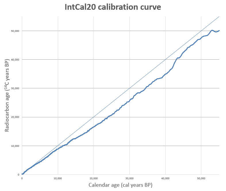
- Raw radiocarbon ages must be converted to calendar years using calibration curves such as IntCal20, which is anchored to dendrochronological records extending back nearly 14,000 years and supplemented by corals, speleothems, and varved sediments to 55,000 years before present.
Radiocarbon dating is a radiometric technique that determines the age of organic materials by measuring the residual concentration of the radioactive isotope carbon-14 (14C). Developed by the American chemist Willard Libby and his colleagues at the University of Chicago in the late 1940s, the method exploits the fact that living organisms continuously exchange carbon with the atmosphere, maintaining an approximately constant ratio of 14C to stable 12C in their tissues, but that this ratio begins to decline through radioactive decay at a known rate once the organism dies.1, 2 Because the half-life of 14C is approximately 5,730 years, the technique is effective for dating materials ranging in age from a few hundred to roughly 50,000 years — a window that encompasses the entirety of recorded human history, the Neolithic transition, the late Pleistocene megafaunal extinctions, and the global dispersal of Homo sapiens.1, 5
Since Libby's initial demonstration, radiocarbon dating has undergone a series of methodological revolutions — from conventional decay counting to accelerator mass spectrometry, from approximate age estimates to high-precision calibrated calendar dates, and from isolated measurements to Bayesian chronological models that integrate multiple lines of evidence. It remains the single most widely used chronometric method in archaeology, paleoclimatology, and Quaternary science, and it has fundamentally reshaped scholarly understanding of when and how key events in human and environmental history occurred.6, 8, 10
Physical basis
Carbon-14 is produced continuously in the upper atmosphere when thermal neutrons generated by cosmic ray interactions collide with nitrogen-14 atoms. In this nuclear reaction, a neutron is captured by the 14N nucleus and a proton is ejected, transforming the nitrogen atom into a 14C atom. The newly formed 14C rapidly oxidizes to carbon dioxide (14CO2), which mixes throughout the atmosphere and enters the biosphere through photosynthesis and the food chain.1, 3 At any given time, approximately one in every 1012 carbon atoms in the atmosphere is 14C, a proportion maintained in a near-steady state by the balance between continuous cosmic-ray production and continuous radioactive decay.1
While an organism is alive, it exchanges carbon with its environment — plants absorb atmospheric CO2 through photosynthesis, animals consume plants or other animals, and marine organisms incorporate dissolved inorganic carbon from seawater. This continuous exchange keeps the 14C/12C ratio in the living organism approximately equal to that of the ambient environment. When the organism dies, however, carbon exchange ceases and the unstable 14C atoms begin to decay without replenishment.1, 2
Carbon-14 decays to nitrogen-14 through beta emission, releasing an electron and an antineutrino. The half-life of this decay — the time required for half the 14C atoms in a sample to transform into 14N — was originally measured by Libby as 5,568 ± 30 years, a value that became conventionally embedded in the field and is still known as the Libby half-life.3 In 1962, Harry Godwin and colleagues published a more accurate determination of 5,730 ± 40 years, subsequently called the Cambridge half-life.4 To maintain comparability across the literature, the radiocarbon community agreed at the 1962 Cambridge conference to continue reporting conventional radiocarbon ages using the Libby half-life, with the understanding that the calibration process would correct for the discrepancy when converting to calendar years.4, 5
Development of the method
The possibility of using 14C as a dating tool was first recognized by Libby in the mid-1940s, building on the 1939 discovery by Serge Korff that cosmic rays produce neutrons in the atmosphere and on earlier theoretical work predicting the existence of 14C as a product of neutron capture by 14N.1, 3 Libby reasoned that if 14C were produced at a roughly constant rate and distributed uniformly through the carbon cycle, then the specific activity of 14C in living organisms should be constant, and the residual activity in dead organisms should decrease predictably with time, serving as a nuclear clock.
The critical first tests came in 1949, when Libby and James Arnold measured the 14C activity of organic samples of known historical age, including wood from the funerary boat of the Egyptian pharaoh Sesostris III (expected age approximately 3,750 years) and wood from the tomb of Zoser at Saqqara (expected age approximately 4,650 years). The radiocarbon ages agreed with the historical ages within the experimental uncertainty, providing powerful validation of the method's fundamental assumptions.2 Libby subsequently extended the technique to a wide range of archaeological and geological materials, and his 1955 monograph Radiocarbon Dating established the protocols that would define the field for decades.1
In 1960, Libby was awarded the Nobel Prize in Chemistry "for his method to use carbon-14 for age determination in archaeology, geology, geophysics, and other branches of science." In his Nobel Lecture, Libby emphasized that the method rested on two fundamental assumptions: that the production rate of 14C in the atmosphere had been essentially constant over the dating range, and that the global carbon cycle mixed 14C rapidly enough to maintain a uniform distribution throughout the biosphere.3 Both assumptions were later shown to be approximations — atmospheric 14C levels have varied significantly over time due to fluctuations in cosmic ray flux, changes in the geomagnetic field, and shifts in the ocean-atmosphere carbon exchange — necessitating the development of calibration curves to convert raw radiocarbon ages to true calendar dates.5, 11
Measurement techniques
Three principal techniques have been used to measure 14C in samples: gas proportional counting, liquid scintillation counting, and accelerator mass spectrometry. Each represents a generational advance in sensitivity, precision, and the minimum sample size required for analysis.
Libby's original method employed a solid carbon sample placed inside a modified Geiger counter, which detected the beta particles emitted by decaying 14C atoms. This approach was soon superseded by gas proportional counting, in which the sample is converted to a gas — typically carbon dioxide or methane — and placed inside a proportional counter that records the ionization events caused by beta decay. Gas counting required several grams of carbon and counting times of one to two days to accumulate sufficient statistics, but it achieved measurement precisions of one to two percent for samples younger than approximately 40,000 years.10, 18
Liquid scintillation counting, developed in the early 1950s and refined through the 1960s and 1970s, converts the sample carbon to benzene, which is mixed with a scintillating solvent. When a 14C atom decays, the emitted beta particle excites the scintillator molecules, producing a flash of light detected by photomultiplier tubes. Liquid scintillation offered comparable precision to gas counting with somewhat easier sample handling, and it became the dominant measurement technique in radiocarbon laboratories from the 1970s through the 1990s.18
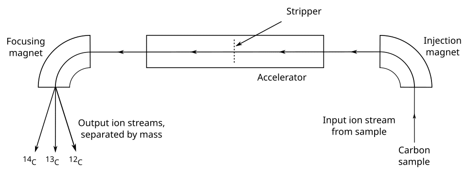
The most transformative advance came with accelerator mass spectrometry (AMS), which was first applied to radiocarbon dating in the late 1970s and became widely available in the 1980s. Rather than waiting for 14C atoms to decay and detecting the resulting radiation, AMS directly counts individual 14C atoms by accelerating carbon ions to high energies and separating them from other isotopes using magnetic and electric fields.6 Because AMS measures the isotope ratio directly rather than the decay rate, it requires roughly one thousand times less material than conventional counting methods — typically 0.5 to 1 milligram of carbon, compared to 1 to 10 grams for decay counting.6, 10 This dramatic reduction in sample size opened entirely new categories of material to radiocarbon dating: individual cereal grains, small bone fragments, single textile fibers, pollen concentrates, and specific chemical compounds extracted from complex matrices. AMS also reduced measurement time from days to hours per sample and extended the practical dating range to approximately 50,000 years before present.6, 10
Comparison of radiocarbon measurement techniques6, 10, 18
| Technique | Era of dominance | Sample size (carbon) | Measurement time | Practical age limit |
|---|---|---|---|---|
| Gas proportional counting | 1950s–1970s | 1–5 g | 1–2 days | ~40,000 yr |
| Liquid scintillation counting | 1970s–1990s | 1–10 g | 1–2 days | ~40,000 yr |
| Accelerator mass spectrometry | 1990s–present | 0.5–1 mg | ~1 hour | ~50,000 yr |
Calibration and the IntCal curves
A raw radiocarbon measurement yields a "conventional radiocarbon age" expressed in years before present (BP, where "present" is defined as 1950 CE by convention), calculated using the Libby half-life and the assumption that atmospheric 14C levels have been constant. In reality, atmospheric 14C concentration has fluctuated significantly over time, driven by changes in the cosmic ray flux modulated by solar activity and the strength of Earth's geomagnetic field, by variations in the rate of ocean-atmosphere carbon exchange, and, in the modern era, by human activities including the burning of fossil fuels (the Suess effect) and atmospheric nuclear weapons testing (the bomb pulse).5, 19 These variations mean that a single radiocarbon age can correspond to multiple calendar dates, or that samples of different true ages can yield the same radiocarbon measurement. Converting a conventional radiocarbon age to a true calendar age therefore requires a calibration curve — an empirically determined record of the relationship between radiocarbon age and calendar age through time.
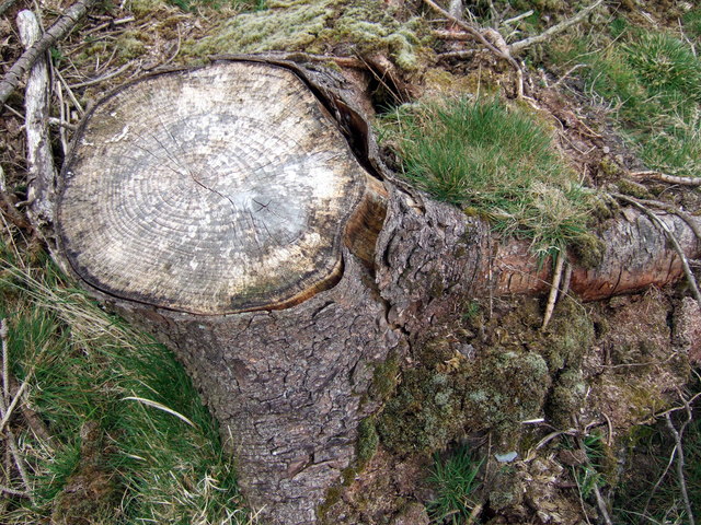
The foundation of radiocarbon calibration is dendrochronology, the science of dating by tree rings. Because each annual growth ring preserves the atmospheric 14C level of the year in which it formed, a continuous tree-ring chronology provides a year-by-year record of past 14C variations. The earliest calibration work used the bristlecone pine chronology of the American Southwest, which extends continuously for more than 8,000 years. Subsequent efforts incorporated oak chronologies from Ireland and Germany, Kauri timber from New Zealand, and other long-lived species, ultimately assembling a dendrochronological record extending back approximately 13,910 calendar years before present.5
Beyond the tree-ring limit, calibration relies on other independently dated archives: uranium-thorium dated corals and speleothems (cave formations), annually laminated (varved) lake and marine sediments, and 14C measurements of plant macrofossils from laminated sequences. The most recent and widely adopted calibration dataset, IntCal20, published in 2020 by an international working group, extends the Northern Hemisphere atmospheric calibration curve to 55,000 calendar years before present with substantially improved resolution and precision compared to its predecessors.5 A companion curve, SHCal20, accounts for the small but significant offset between Northern and Southern Hemisphere atmospheric 14C levels caused by the greater ocean surface area in the Southern Hemisphere, which draws down more 14CO2 from the atmosphere.15
The calibration process involves comparing the measured radiocarbon age and its associated uncertainty against the calibration curve to produce a probability distribution of possible calendar ages. Because the calibration curve is not monotonic — periods of relatively constant or fluctuating atmospheric 14C can create plateaux and wiggles — a single radiocarbon measurement can yield a broad, multimodal calendar age distribution, particularly during certain intervals such as the Hallstatt plateau (approximately 800–400 BCE) where the calibration curve is nearly flat.5, 8
Sources of error and complications
Several systematic effects can cause radiocarbon dates to diverge from the true age of the event of archaeological interest. Understanding and mitigating these effects is essential to the reliable application of the method.
The marine reservoir effect arises because the ocean contains a large reservoir of dissolved inorganic carbon that is significantly depleted in 14C relative to the atmosphere, owing to the slow mixing of surface waters with 14C-depleted deep water that has been isolated from the atmosphere for centuries. Organisms that derive their carbon from seawater — marine shells, fish, sea mammals, and seabirds — therefore yield radiocarbon ages that are systematically older than contemporaneous terrestrial samples. The global average marine reservoir offset is approximately 400 years, but the local deviation from this average, designated ΔR, varies considerably with geography, ocean circulation patterns, and upwelling intensity, ranging from near zero in some tropical Atlantic locations to more than 800 years in Arctic and Antarctic waters.9, 23 The Marine20 calibration curve, published alongside IntCal20, provides a modeled global average marine calibration, but site-specific ΔR corrections remain essential for accurate dating of marine-influenced samples.23
The old wood effect refers to the discrepancy between the radiocarbon age of a piece of wood or charcoal and the date of the archaeological event it is supposed to represent. The heartwood of a tree ceases exchanging carbon with the atmosphere decades or centuries before the tree is felled, so a radiocarbon date on inner wood from a long-lived species reflects the year the ring grew, not the year the tree was cut or the wood was used. This inbuilt age is compounded when old timber is reused, salvaged, or curated, potentially introducing offsets of centuries or, in extreme cases, millennia. Archaeologists mitigate the old wood effect by preferentially selecting short-lived materials for dating: annual seeds, cereal grains, nutshells, small twigs, or the outermost rings of timbers with preserved bark.14, 17
Contamination — the introduction of carbon that is not original to the sample — is the most insidious source of error. Even a small amount of modern carbon can dramatically affect the apparent age of an old sample: 1 percent modern carbon contamination will shift a 34,000-year-old sample by approximately 4,000 years toward the present. Contamination sources include humic acids from soil, calcium carbonate from groundwater, consolidants applied during excavation or museum conservation, and modern handling without gloves.7, 14 To remove contaminants, radiocarbon laboratories apply rigorous chemical pretreatment protocols before measurement. The most common protocol for charcoal and plant material is the acid-base-acid (ABA) sequence, which uses hydrochloric acid to remove carbonates, sodium hydroxide to dissolve humic acids, and a final acid wash to remove atmospheric CO2 absorbed during the base step. For older or more contaminated charcoals, the more aggressive ABOx-SC (acid-base-oxidation–stepped combustion) protocol applies a potassium dichromate oxidation step followed by a controlled stepped combustion to isolate the most resistant carbonaceous fraction.14, 17
For bone samples, the primary dating target is collagen, the structural protein that constitutes roughly 20 percent of fresh bone by weight but degrades progressively in burial environments. The Oxford Radiocarbon Accelerator Unit pioneered the ultrafiltration protocol, in which extracted collagen is passed through a molecular filter that retains only the high-molecular-weight fraction (greater than 30 kilodaltons), excluding degraded collagen fragments and low-molecular-weight contaminants. When applied to Palaeolithic-age bone, ultrafiltration has repeatedly produced ages that are significantly older than previous measurements on the same samples, demonstrating that earlier dates were systematically too young due to incomplete removal of contaminants.7, 13
Effective dating range
The practical upper limit of radiocarbon dating is governed by the decreasing abundance of 14C atoms in progressively older samples. After approximately 10 half-lives (roughly 57,300 years), the residual 14C activity falls below one-thousandth of the modern level, making it extremely difficult to distinguish the sample signal from background radiation in the measurement apparatus. For conventional decay-counting methods, the practical limit was approximately 40,000 years. AMS, with its superior sensitivity to low 14C/12C ratios, has extended this to approximately 50,000 years, and under optimal conditions with very large samples and extended counting times, some laboratories have reported measurements approaching 55,000 to 60,000 years, though the uncertainties on such dates are large.6, 10, 11
At the young end of the scale, radiocarbon dating is complicated by two twentieth-century anthropogenic perturbations. The Suess effect, identified by Hans Suess in 1954, refers to the dilution of atmospheric 14C by the combustion of fossil fuels, which release vast quantities of 14C-free carbon dioxide. By the mid-twentieth century, this effect had measurably lowered atmospheric 14C levels, mimicking the decay signature and making very recent samples appear slightly older than their true age.19 In the opposite direction, atmospheric nuclear weapons testing between 1945 and 1963 nearly doubled the concentration of 14C in the atmosphere, creating the so-called bomb pulse. Since the 1963 Limited Test Ban Treaty, the excess atmospheric 14C has been declining as it is absorbed into the ocean and biosphere. The bomb pulse, while complicating conventional radiocarbon dating of very recent materials, has found applications in forensic science, cell biology, and environmental tracer studies, because any organic material formed after 1955 carries a distinctly elevated 14C signature that can be used to determine its year of formation with high precision.10
Approximate residual 14C after successive half-lives1, 4
Bayesian chronological modeling
A single calibrated radiocarbon date often produces a broad probability distribution that spans centuries, particularly during periods when the calibration curve is flat or oscillating. In archaeological practice, however, radiocarbon dates are rarely interpreted in isolation. They are associated with stratigraphic sequences, typological orderings, and historical constraints that carry independent chronological information. Bayesian chronological modeling provides a formal statistical framework for integrating these multiple lines of evidence, combining the likelihood of the radiocarbon measurements with prior information about the relative ordering, grouping, and tempo of events to produce posterior probability distributions that are substantially more precise than the individual calibrated dates alone.8, 22
The development of Bayesian methods for radiocarbon dating was pioneered by Caitlin Buck and colleagues in the early 1990s and implemented in widely used software packages, most notably OxCal, created and maintained by Christopher Bronk Ramsey at the University of Oxford.8, 22 In a typical Bayesian model, the archaeologist specifies the stratigraphic relationships among dated samples (for example, that sample A must be older than sample B because it was found in a lower layer) and groups them into phases or sequences that reflect the site's depositional history. The model then uses Markov chain Monte Carlo algorithms to sample from the joint posterior distribution, yielding refined calendar age estimates for each date and, critically, for the boundaries of phases — the estimated dates at which activities began or ended.8
Bayesian modeling has proven especially powerful for questions about the timing and duration of cultural transitions. By modeling large numbers of radiocarbon dates from multiple sites within a Bayesian framework, researchers can estimate when a particular innovation, such as the adoption of agriculture or the introduction of a new ceramic tradition, first appeared in a region, how rapidly it spread, and when it became dominant. The approach has transformed radiocarbon dating from a technique that produces isolated age measurements into a tool for constructing detailed event histories with quantified uncertainties.8, 22
Applications in archaeology
Radiocarbon dating has contributed to virtually every major chronological question in the archaeology and paleoanthropology of the past 50,000 years. Several applications illustrate the scope and transformative impact of the method.
The timing of the Neolithic transition — the shift from hunting and gathering to farming — was one of the first archaeological problems to be illuminated by radiocarbon. In a landmark study, Albert Ammerman and Luigi Luca Cavalli-Sforza compiled radiocarbon dates from early Neolithic sites across Europe and demonstrated that farming spread from the Near East to northwestern Europe in a wave-of-advance pattern at a rate of approximately one kilometre per year, arriving in Greece by around 7000 BCE and reaching the British Isles and Scandinavia by around 4000 BCE.12 Subsequent work with much larger databases and Bayesian modeling has refined this picture, revealing that the spread was neither uniform nor continuous but involved leapfrog movements, periods of stasis, and regionally variable rates that depended on environmental conditions and the existing population of hunter-gatherers.20
The radiocarbon chronology of the Middle to Upper Palaeolithic transition — the period during which Neanderthals disappeared and anatomically modern humans became the sole hominin species in Europe — has been dramatically revised by improved pretreatment methods. Redating of key Neanderthal specimens from Belgium using compound-specific radiocarbon analysis demonstrated that the bones were 44,200 to 40,600 calendar years old, thousands of years older than previous measurements had indicated and consistent with a more rapid replacement of Neanderthals across Europe than earlier chronologies suggested.13 Similarly, the application of the ABOx-SC pretreatment protocol to charcoal from Palaeolithic cave sites in Iberia overturned earlier claims that Neanderthals had survived in southern refugia until as recently as 28,000 years ago, instead demonstrating that most of the purportedly late Neanderthal dates were artifacts of contamination.17
Radiocarbon dating has also clarified the timing of late Pleistocene megafaunal extinctions. In New Zealand, where the arrival of Polynesian settlers and the extinction of the moa (large flightless birds) occurred within the narrow historical window of the last millennium, high-precision radiocarbon dating of moa bones and associated archaeological deposits demonstrated that all moa species became extinct within approximately 100 years of initial human contact, around 1400 CE — one of the most rapid, well-documented cases of human-caused extinction.21
In the realm of historical archaeology, radiocarbon dating has provided independent chronological control for objects of disputed age. The 1988 dating of the Shroud of Turin by three independent AMS laboratories yielded calibrated dates of 1260–1390 CE, placing the cloth firmly in the medieval period rather than the first century CE.16 This study demonstrated both the precision achievable by AMS and the power of radiocarbon dating to resolve long-standing historical controversies with objective physical measurements.
Current frontiers
Contemporary radiocarbon research continues to push the boundaries of precision, resolution, and applicability. The development of compound-specific radiocarbon analysis — in which individual amino acids or lipids are isolated from a complex sample and dated separately — represents the latest advance in pretreatment methodology. By targeting a single molecular species (typically hydroxyproline, an amino acid found almost exclusively in collagen), this approach eliminates contamination from non-collagenous carbon sources more effectively than bulk collagen methods and has yielded revised ages for some of the most contested specimens in Palaeolithic archaeology.10, 13
Improvements in AMS instrumentation continue to enhance sensitivity and throughput. Modern facilities equipped with multi-cathode ion sources can process hundreds of samples per day, while advances in carbon preparation have further reduced the minimum sample size to as little as 20 micrograms of carbon for some applications.10 The extension of the IntCal calibration curve to 55,000 years before present has provided, for the first time, a continuous and internally consistent calibration framework spanning the entire effective range of radiocarbon dating, enabling more reliable age estimates for the critical period of the late Middle Palaeolithic and the earliest Upper Palaeolithic.5, 11
The integration of radiocarbon with other dating methods — optically stimulated luminescence, uranium-series dating, tephrochronology, and palaeomagnetic stratigraphy — within unified Bayesian models is becoming standard practice for complex archaeological and palaeoenvironmental sequences. These multi-method chronological frameworks, anchored by the high precision of calibrated radiocarbon dates and supported by the independent age constraints of other techniques, represent the current state of the art in archaeological chronology and promise further refinements as calibration data, pretreatment protocols, and statistical methodologies continue to improve.8, 10, 22
References
The worldwide marine radiocarbon reservoir effect: definitions, mechanisms, and prospects
Developments in radiocarbon technologies: from the Libby counter to compound-specific AMS analyses
Current pretreatment methods for AMS radiocarbon dating at the Oxford Radiocarbon Accelerator Unit (ORAU)
Radiocarbon dating casts doubt on the late chronology of the Middle to Upper Palaeolithic transition in southern Iberia
Radiocarbon evidence for the timing of megafaunal extinction in New Zealand and the Chatham Islands