Overview
- Stratigraphy is the science of interpreting rock layers and their relationships, built on foundational principles articulated by Nicolaus Steno in 1669 and refined over three centuries into a family of complementary subdisciplines — lithostratigraphy, biostratigraphy, chronostratigraphy, magnetostratigraphy, chemostratigraphy, and sequence stratigraphy — that together provide the temporal framework for all of Earth history.
- The Global Boundary Stratotype Section and Point (GSSP) system, maintained by the International Commission on Stratigraphy, anchors the geologic time scale to physical reference sections in rock outcrops around the world, with 81 of 101 stage boundaries now formally ratified.
- Modern stratigraphy integrates fossil zones, magnetic polarity reversals, stable isotope excursions, and sequence-bounding unconformities to correlate rock sequences across continents and ocean basins at resolutions approaching tens of thousands of years, enabling precise reconstruction of past climates, sea levels, and biological evolution.
Stratigraphy is the branch of geology concerned with the description, classification, and interpretation of layered rocks and their relationships to one another and to geologic time. The discipline rests on a set of geometric principles first articulated in the seventeenth century, which hold that sedimentary strata are deposited in predictable spatial and temporal patterns that can be read to reconstruct the history of the Earth. Over the past three and a half centuries, stratigraphy has evolved from a qualitative exercise in ordering rock layers into a sophisticated, multi-method science that integrates fossil content, rock type, magnetic polarity, chemical composition, and depositional architecture to build a unified temporal framework for the planet's 4.54-billion-year history.1, 2 That framework — the geologic time scale — is stratigraphy's most consequential product, and every division within it, from eon to age, is ultimately defined by relationships observable in rock.
Steno's principles and classical foundations
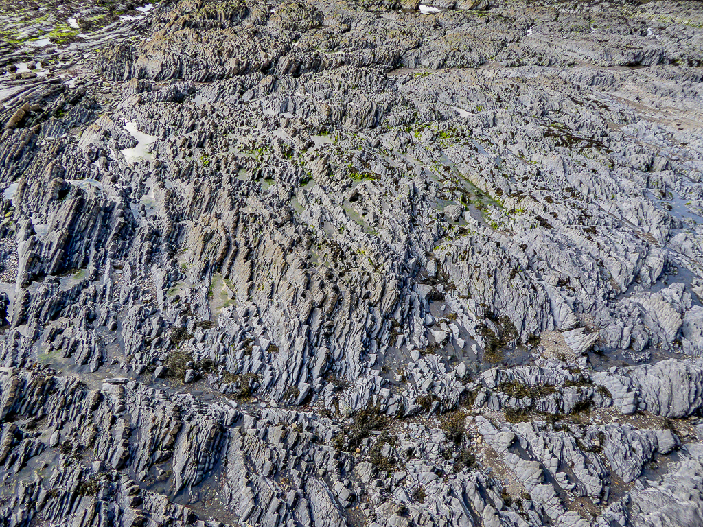
The intellectual foundations of stratigraphy were laid by the Danish anatomist and natural philosopher Nicolaus Steno (Niels Stensen) in his 1669 treatise De Solido Intra Solidum Naturaliter Contento Dissertationis Prodromus.1 Working in Tuscany, Steno examined the rock layers exposed in hillsides and quarries and articulated three principles that remain the logical bedrock of stratigraphic reasoning. The principle of superposition states that in any undisturbed succession of strata, each layer is younger than the one beneath it and older than the one above. The principle of original horizontality states that layers of sediment are deposited in a nearly horizontal position; if strata are found tilted, folded, or overturned, they have been deformed by subsequent tectonic forces. The principle of lateral continuity holds that a stratum, at the time of its deposition, extended continuously in all directions until it thinned to nothing or terminated against the margin of the depositional basin.1, 2
These three axioms were later supplemented by the principle of cross-cutting relationships, which holds that any geological feature — a fault, an igneous intrusion, an erosion surface — that cuts across pre-existing strata must be younger than those strata.3 James Hutton's recognition in 1788 of angular unconformities in the Scottish landscape demonstrated that the rock record contains profound temporal gaps: surfaces where older, deformed strata were eroded flat before younger, horizontal layers were deposited atop them.17 The implication that enormous stretches of time must have elapsed during the formation, deformation, erosion, and re-burial of rock was among the first intimations of deep time in the geological sciences. Together, these principles allow geologists to establish the relative age of rocks in any exposure, even without knowledge of their absolute age in years.
Lithostratigraphy
Lithostratigraphy is the subdivision of the rock record based on the observable physical properties of rock units — their lithology, texture, color, mineralogy, and bedding characteristics — rather than their age or fossil content. It is the most fundamental and field-accessible branch of stratigraphy, and its units form the basic mapping vocabulary of geological survey work worldwide.7, 8
The primary unit of lithostratigraphy is the formation, defined as a body of rock sufficiently distinctive in lithological character and sufficiently thick to be mappable at the surface or traceable in the subsurface. Formations are given geographic names drawn from the locality where they were first described or where they are especially well exposed — for example, the Morrison Formation (Jurassic fluvial and lacustrine sediments of the western United States) or the Chalk (Upper Cretaceous marine carbonate of northwestern Europe). Formations may be grouped into larger units called groups when two or more formations share a general lithological character or a common depositional history, or subdivided into members and beds when finer distinctions are useful.7
A critical feature of lithostratigraphic units is that they are explicitly time-transgressive: a formation defined by a particular rock type may have been deposited at different times in different places as the environment that produced it migrated across the landscape. A sandy shoreline deposit, for instance, shifts landward during a marine transgression, so the resulting sandstone formation is progressively younger inland. Lithostratigraphy therefore tells geologists what kind of rock is present and where, but it does not directly indicate when that rock was deposited. For temporal information, geologists turn to biostratigraphy and chronostratigraphy.2, 8
Biostratigraphy
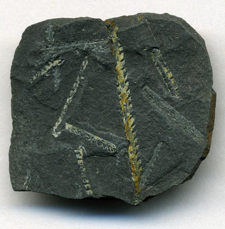
Biostratigraphy uses the fossil content of sedimentary rocks to subdivide and correlate strata. The method is grounded in the principle of faunal succession, developed empirically by the English canal surveyor William Smith in the early nineteenth century, which holds that fossil assemblages succeed one another in a definite and recognizable order through the stratigraphic column.4 Smith demonstrated that each stratum in the sequence of rocks exposed across England contained a characteristic set of fossils, and that these fossil assemblages could be used to identify and correlate that stratum over great distances, even where the lithology changed. His 1815 geological map of England and Wales, the first of its kind, was a direct product of this biostratigraphic insight.4
The fundamental unit of biostratigraphy is the biozone (or zone), defined by the range or association of one or more fossil taxa. Several types of biozones are recognized. A range zone encompasses the total vertical (temporal) range of a single taxon. A concurrent range zone (or overlap zone) is the stratigraphic interval in which two or more taxa co-occur, often providing finer resolution than any single taxon's range. An interval zone is defined by the strata between two biohorizons, such as the first appearance datum (FAD) of one species and the FAD of another. An assemblage zone is defined by a distinctive association of three or more taxa that, taken together, distinguish it from adjacent zones.5, 9
The most useful biostratigraphic fossils, commonly called index fossils or guide fossils, share several properties: they are abundant, geographically widespread, morphologically distinctive, easy to identify, and have short stratigraphic (temporal) ranges. Organisms that satisfy these criteria include graptolites in the Ordovician and Silurian, ammonites in the Jurassic and Cretaceous, conodonts across much of the Paleozoic, and planktonic foraminifera and calcareous nannofossils in the Mesozoic and Cenozoic. The zonation schemes built from these groups remain indispensable for dating and correlating sedimentary sequences, particularly in marine settings where continuous deposition has preserved long, fossil-rich records.5, 6
Selected index fossil groups and their stratigraphic utility5, 6
| Fossil group | Useful range | Typical zone duration | Environment |
|---|---|---|---|
| Trilobites | Cambrian–Ordovician | ~2–5 Myr | Marine |
| Graptolites | Ordovician–Silurian | ~0.5–2 Myr | Marine (pelagic) |
| Conodonts | Cambrian–Triassic | ~0.5–3 Myr | Marine |
| Ammonites | Devonian–Cretaceous | ~0.5–1 Myr | Marine |
| Planktonic foraminifera | Jurassic–present | ~0.3–1 Myr | Marine (pelagic) |
| Calcareous nannofossils | Jurassic–present | ~0.3–2 Myr | Marine (pelagic) |
| Pollen and spores | Silurian–present | ~1–5 Myr | Terrestrial & nearshore |
Chronostratigraphy and the time scale
Chronostratigraphy is the branch of stratigraphy that organizes rock into units corresponding to intervals of geologic time. Whereas lithostratigraphy classifies rock by its physical properties and biostratigraphy classifies it by its fossil content, chronostratigraphy classifies it by when it was deposited. The chronostratigraphic hierarchy consists of nested units of decreasing duration: eonothems, erathems, systems, series, and stages, each corresponding to a named interval on the geologic time scale (eons, eras, periods, epochs, and ages, respectively).5, 8
The stage is the smallest formally defined chronostratigraphic unit and typically corresponds to an interval of a few million years. Stages are the building blocks from which all higher-order divisions of the time scale are constructed. The Maastrichtian Stage, for example, is the uppermost stage of the Cretaceous System; it spans approximately 72.1 to 66.0 million years ago and is defined by specific biostratigraphic and magnetostratigraphic criteria at its base.6, 20 Stages are grouped into series (corresponding to epochs), series into systems (periods), systems into erathems (eras), and erathems into eonothems (eons). The boundaries between these units are positioned at major shifts in the fossil record, geochemical signatures, or magnetic polarity, typically corresponding to evolutionary turnover events, mass extinctions, or significant environmental transitions.5
A fundamental principle of chronostratigraphy is that its boundaries are defined at their base. Each stage is defined by the characteristics at its lower boundary; its upper boundary is automatically the base of the next-younger stage. This convention eliminates ambiguity and ensures that the entire rock record is partitioned into a continuous series of non-overlapping units with no gaps or duplications.8, 18
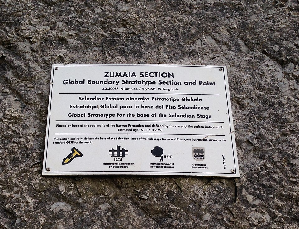
The GSSP system
The mechanism by which chronostratigraphic boundaries are made precise and internationally reproducible is the Global Boundary Stratotype Section and Point, or GSSP — colloquially known as the "golden spike."
To be ratified, a GSSP candidate must satisfy a set of stringent requirements. The section must be continuously exposed and accessible, with no significant structural disturbance or metamorphic overprint. It must contain an adequate record of the primary correlation event — typically a biostratigraphic first appearance, a magnetic polarity reversal, or a geochemical excursion — together with multiple auxiliary markers that allow the boundary to be recognized in sections elsewhere. The section should be amenable to radiometric dating, or at least to calibration against a well-dated reference section, and it must be in a geologically stable setting where long-term preservation is expected.6, 18
As of 2025, 81 of the 101 stages that require a GSSP have been formally ratified. The Ordovician, Silurian, and Devonian systems are the only ones in which every stage boundary has a ratified GSSP. Several Precambrian and Cambrian boundaries remain formally undefined, in part because the fossil record is sparser and the rocks are more commonly metamorphosed or deformed, making it difficult to identify continuously exposed sections with adequate marker events.6 The GSSP system replaced an older practice of defining boundaries by "type areas" or "type sections" that were often geographically and stratigraphically vague. By anchoring each boundary to a single physical point in rock, the GSSP approach has made the geologic time scale an empirically grounded, internationally standardized reference framework.18
Magnetostratigraphy
Magnetostratigraphy exploits the fact that Earth's magnetic field has reversed its polarity hundreds of times over geologic history, and that sedimentary and volcanic rocks record the ambient field direction at the time of their formation. Iron-bearing mineral grains in sediment align with the geomagnetic field as they settle through the water column or shortly after deposition, and this natural remanent magnetization (NRM) is locked in during lithification. By sampling a stratigraphic section at closely spaced intervals and measuring the polarity of the NRM in each sample, geologists can construct a local magnetic polarity stratigraphy — a sequence of normal- and reversed-polarity zones that can be correlated with the global geomagnetic polarity time scale (GPTS).10, 11
The GPTS was originally constructed from the pattern of magnetic anomalies on the ocean floor, where the symmetric stripe pattern of normal and reversed polarity on either side of mid-ocean ridges preserves a continuous record of geomagnetic reversals extending back to approximately 170 million years ago. The most widely used calibration of this pattern is that of Cande and Kent (1995), who tied the anomaly sequence to radiometrically dated tie points to produce a polarity time scale for the Late Cretaceous and Cenozoic with a resolution of a few hundred thousand years.10 Subsequent refinements using astronomical tuning — the calibration of polarity boundaries against the astronomically paced rhythms of Milankovitch climate cycles recorded in deep-sea sediments — have pushed the precision of certain intervals below 100,000 years.6, 20
Magnetostratigraphy is especially valuable where biostratigraphic markers are absent or poorly preserved, such as in continental red beds, lacustrine sediments, and volcaniclastic sequences. Because geomagnetic reversals are globally synchronous and independent of environment or facies, a well-resolved polarity stratigraphy can correlate marine and terrestrial sections that share no fossil taxa in common. Magnetostratigraphy has been instrumental in calibrating the hominin fossil record of East Africa, where sequences of volcanic ash and fluvial sediments interbedded with fossiliferous horizons have been dated by matching their polarity patterns to the GPTS.11
Chemostratigraphy
Chemostratigraphy uses systematic variations in the chemical and isotopic composition of sedimentary rocks as tools for stratigraphic correlation and paleoenvironmental reconstruction. The approach is founded on the principle that the chemistry of seawater, and by extension the chemistry of minerals precipitated from it, varies through time in response to global-scale changes in tectonics, volcanism, weathering, biological productivity, and ocean circulation. If these variations are sufficiently large and rapid, they can serve as stratigraphic markers analogous to biostratigraphic first appearances or magnetic polarity reversals.12, 13
The two most widely applied chemostratigraphic proxies are carbon isotopes (δ13C) and strontium isotopes (87Sr/86Sr). The carbon isotope ratio of marine carbonates reflects the balance between organic carbon burial (which preferentially removes the lighter isotope 12C, driving seawater δ13C to more positive values) and volcanic or metamorphic degassing (which returns isotopically light carbon to the ocean-atmosphere system). Large positive and negative δ13C excursions recorded in carbonate rocks have been correlated globally and tied to major events in Earth history, including the Neoproterozoic glaciations, the end-Permian mass extinction, and the Paleocene-Eocene Thermal Maximum.22
Strontium isotope stratigraphy takes advantage of the fact that the 87Sr/86Sr ratio of seawater has varied monotonically over certain intervals of the Phanerozoic, making it possible to assign a numerical age to a marine carbonate sample by measuring its strontium isotope ratio and comparing it to the well-calibrated global 87Sr/86Sr curve. The approach is most powerful during intervals when the curve changes rapidly and unidirectionally, as in the Cenozoic, where strontium isotope ratios have risen steeply as the collision of India with Asia exposed vast areas of radiogenic continental crust to chemical weathering. The comprehensive Phanerozoic seawater 87Sr/86Sr curve compiled by Veizer and colleagues (1999), based on more than 4,000 calcite shell analyses, remains a foundational reference for this method.12, 21
Other chemostratigraphic tools include sulfur isotopes (δ34S), which track changes in the marine sulfur cycle and redox conditions; oxygen isotopes (δ18O), which record temperature and ice-volume changes; and elemental abundance ratios such as Fe/Al and Mn/Al, which serve as proxies for redox state and hydrothermal input. Chemostratigraphy is particularly valuable in Precambrian sequences, where the fossil record is sparse and biostratigraphy has limited applicability. Major carbon isotope excursions in the Neoproterozoic have become primary tools for correlating successions that predate the evolution of most index fossil groups.13, 22
Sequence stratigraphy
Sequence stratigraphy analyzes the sedimentary record as a series of genetically related packages of strata — called depositional sequences — bounded by unconformities and their correlative conformities. The approach was pioneered in the 1960s by L. L. Sloss, who recognized continent-wide unconformity-bounded sequences in the cratonic interior of North America, and formalized in the late 1970s by Peter Vail, Robert Mitchum, and colleagues at Exxon Production Research Company, who used seismic reflection profiles to demonstrate that sedimentary basins worldwide record a broadly synchronous pattern of sequence-bounding unconformities driven by changes in relative sea level.14, 19
Within each sequence, geologists recognize subdivisions called systems tracts, each representing a distinct phase of the sea-level cycle. A lowstand systems tract forms when relative sea level is lowest and rivers incise into the exposed shelf, delivering sediment to the basin floor. A transgressive systems tract develops during rapid sea-level rise, when the shoreline retreats landward and fine-grained condensed sections accumulate on the outer shelf. A highstand systems tract forms when the rate of sea-level rise slows and sediment progrades seaward across the shelf. These systems tracts are separated by key surfaces: the sequence boundary (an unconformity or its correlative conformity), the transgressive surface, and the maximum flooding surface.15, 16
The relative contributions of eustasy (global sea-level change), tectonic subsidence, and sediment supply to any given sequence remain a subject of active investigation. The original Exxon model emphasized global eustatic control, but subsequent work has shown that local tectonics and sediment supply can amplify, suppress, or even generate sequence boundaries independently of eustatic change. Modern sequence stratigraphy therefore evaluates each of these controls independently for each basin, rather than assuming a single global signal.16
Integrated stratigraphy and modern practice
The power of modern stratigraphy lies not in any single method but in the integration of multiple independent datasets. A well-characterized stratigraphic section today typically includes a lithological log (lithostratigraphy), a fossil zonation (biostratigraphy), a magnetic polarity column (magnetostratigraphy), one or more isotopic profiles (chemostratigraphy), and a depositional model (sequence stratigraphy), all calibrated where possible against radiometric ages.5, 6, 23 This integrated approach allows each method to compensate for the limitations of the others: biostratigraphy provides high-resolution dating where fossils are abundant but fails in unfossiliferous rocks; magnetostratigraphy provides globally synchronous markers but requires independent calibration to distinguish one reversal from another; chemostratigraphy correlates across facies boundaries but can be compromised by diagenesis; radiometric dating provides absolute ages but is applicable only where datable minerals are present.
Approximate temporal resolution of major stratigraphic methods5, 6, 10
The ongoing refinement of the geologic time scale is a direct product of this integrative work. Each new GSSP ratification, each new radiometric age for a polarity reversal or a biostratigraphic datum, and each new isotopic curve tightens the calibration of the stratigraphic framework and improves the temporal resolution with which geologists can reconstruct events in deep time. The International Chronostratigraphic Chart, maintained by the International Commission on Stratigraphy, is updated regularly to incorporate these advances and serves as the primary reference for the scientific community worldwide.5, 6 Stratigraphy, in this sense, is not a static classification scheme but a living, continuously improving record of the planet's history, built layer by layer from the rocks themselves.
References
Memoir to the Map and Delineation of the Strata of England and Wales, with Part of Scotland
International Stratigraphic Guide: A Guide to Stratigraphic Classification, Terminology, and Procedure
Revised calibration of the geomagnetic polarity timescale for the Late Cretaceous and Cenozoic
Seismic Stratigraphy and Global Changes of Sea Level: Part 3. Relative Changes of Sea Level from Coastal Onlap