Overview
- The Hertzsprung–Russell diagram, developed independently by Ejnar Hertzsprung (1905–1911) and Henry Norris Russell (1913–1914), plots stellar luminosity against surface temperature or spectral type and remains the single most important organizational tool in stellar astrophysics, encoding the evolutionary state of every star in one compact visualization.
- The Harvard spectral classification system—OBAFGKM, refined by Annie Jump Cannon and rooted in the ionization physics formalized by Meghnad Saha’s 1920 equation—provides the temperature axis, while the Morgan–Keenan luminosity classes (I through V) add a second dimension that distinguishes giants from dwarfs at the same spectral type and enables spectroscopic distance determination.
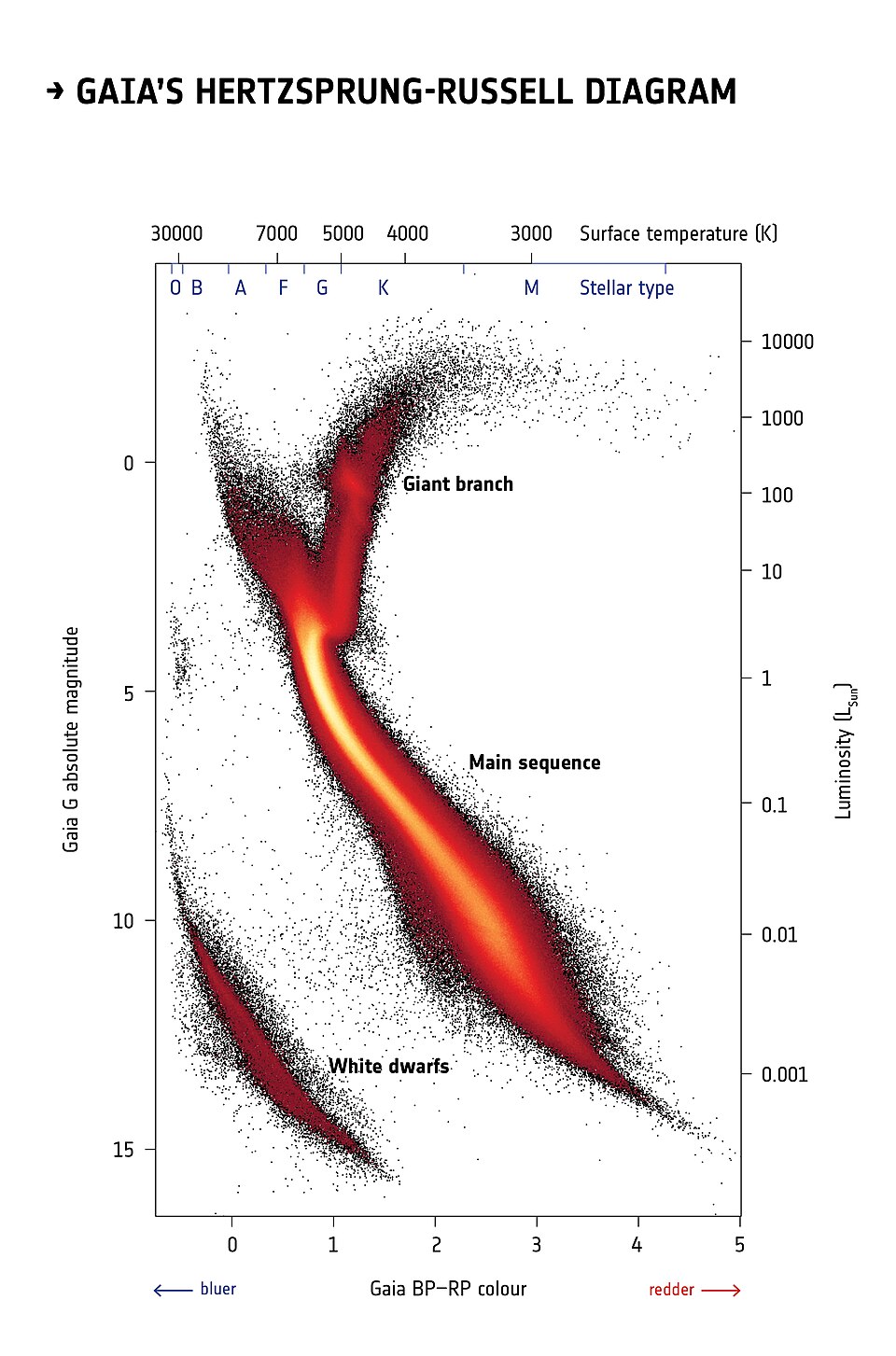
- Modern extensions include the L, T, and Y spectral classes for brown dwarfs cooler than M stars, and the ESA Gaia mission has produced precision HR diagrams for over a billion stars, revealing fine structure in the main sequence, white dwarf cooling tracks, and metal-poor subdwarf populations with unprecedented clarity.
The Hertzsprung–Russell diagram is the single most important graphical tool in stellar astrophysics. By plotting the intrinsic luminosity of a star against its surface temperature or spectral type, the diagram reveals that stars are not scattered at random across parameter space but instead cluster into well-defined regions that correspond to distinct physical states and evolutionary phases. The main sequence, the red giant branch, the horizontal branch, the asymptotic giant branch, and the white dwarf cooling sequence all occupy characteristic locations on this plot, so that a star's position on the diagram immediately conveys information about its mass, age, internal structure, and ultimate fate.11, 12
The diagram emerged from two independent lines of investigation in the early twentieth century and has been refined continuously ever since—from the Harvard spectral classification and the Morgan–Keenan luminosity classes to modern extensions encompassing brown dwarfs and the precision astrometry of the ESA Gaia mission. Understanding the HR diagram is prerequisite to understanding stellar evolution itself, because the diagram is both the observational summary of what stars do and the primary testing ground against which theoretical models are evaluated.5, 16
Historical development
The conceptual foundation of the HR diagram was laid by the Danish astronomer Ejnar Hertzsprung. In 1905, Hertzsprung published a paper in the Zeitschrift für wissenschaftliche Photographie—a journal of photographic science that few astronomers read—in which he analyzed the photometric properties of stars classified by the Harvard spectral system. He demonstrated that stars of spectral types G, K, and M fell into two distinct populations: a majority of faint, nearby objects and a minority of enormously luminous, distant ones. Hertzsprung had discovered the distinction between dwarf and giant stars, a division that would become one of the defining features of the diagram that bears his name.1, 5
In 1911, Hertzsprung published more extensive photometric work based on photographic effective wavelengths of stars in the Pleiades and Hyades clusters, plotted against their apparent magnitudes. Because stars in a given cluster are all at approximately the same distance, differences in apparent magnitude correspond directly to differences in intrinsic luminosity, making clusters ideal laboratories for revealing correlations between color and brightness. These 1911 diagrams, published in the Publikationen des Astrophysikalischen Observatoriums zu Potsdam, constitute the earliest recognizable versions of the HR diagram, although their publication in a relatively obscure venue limited their immediate impact.2, 5
The American astronomer Henry Norris Russell arrived at the same insight independently and with far greater visibility. Drawing on trigonometric parallax measurements that provided direct distance estimates for nearby stars, Russell constructed a plot of absolute magnitude against spectral type for a large sample of field stars. He presented this diagram in December 1913 at a joint meeting of the American Astronomical Society and the American Association for the Advancement of Science in Atlanta, Georgia, and published the results in 1914 in both Popular Astronomy and Nature.3, 4 Russell's diagram clearly showed the main sequence running diagonally from hot, luminous stars to cool, faint ones, with a separate population of luminous red giants offset to the upper right. Because Russell's work reached a much wider audience and rested on parallax-based absolute magnitudes rather than cluster photometry alone, it established the diagram as a central tool of stellar astronomy. The combined designation "Hertzsprung–Russell diagram" was adopted to recognize both pioneers' contributions.5
Spectral classification in detail
The horizontal axis of the HR diagram is provided by spectral classification, a system whose development was one of the great collective achievements of late nineteenth- and early twentieth-century astronomy. The work was carried out primarily at the Harvard College Observatory, where Edward C. Pickering directed a program to photograph and classify the spectra of tens of thousands of stars as part of the Henry Draper Memorial, funded by a bequest from the widow of the physician and amateur astronomer Henry Draper.6
The classification was performed largely by a group of women astronomers known informally as the "Harvard Computers." Among them, Annie Jump Cannon made the most enduring contribution. Building on earlier work by Williamina Fleming and Antonia Maury, Cannon streamlined the classification scheme into the sequence O, B, A, F, G, K, M, ordered by decreasing surface temperature rather than by the original alphabetical labels. Each class was further subdivided into ten numerical subtypes (0 through 9), yielding a finely graded temperature scale. Cannon personally classified the spectra of over 350,000 stars for the Henry Draper Catalogue, published in nine volumes between 1918 and 1924. In 1922, the International Astronomical Union formally adopted her classification system, and with only minor extensions it remains the standard today.6
The physical explanation for why different spectral types display different absorption lines came with the application of atomic physics to stellar atmospheres. In 1920, the Indian physicist Meghnad Saha derived an equation relating the ionization state of a gas in thermal equilibrium to its temperature and electron pressure.7 The Saha equation showed that the pattern of absorption lines in a stellar spectrum is determined primarily by the temperature and pressure of the stellar atmosphere, not by differences in chemical composition. At high temperatures, atoms are highly ionized and the absorption lines of neutral species weaken; at low temperatures, molecules can form and dominate the spectrum. The spectral sequence OBAFGKM thus corresponds to a monotonic decrease in surface temperature from roughly 50,000 kelvins for the hottest O-type stars to below 3,000 kelvins for the coolest M dwarfs.7, 11
In 1925, Cecilia Payne (later Payne-Gaposchkin) applied the Saha equation systematically in her doctoral thesis at Harvard, demonstrating that the enormous variation in stellar spectra along the OBAFGKM sequence could be explained almost entirely by temperature differences while the underlying chemical composition was remarkably uniform—dominated overwhelmingly by hydrogen and helium. Her thesis, described by Otto Struve as "the most brilliant PhD thesis ever written in astronomy," established that the spectral classification sequence is fundamentally a temperature sequence.8
Properties of the main spectral classes11, 12
| Spectral class | Surface temperature (K) | Color | Key absorption features | Example star |
|---|---|---|---|---|
| O | >30,000 | Blue | He II, N III, C III; weak H lines | 10 Lacertae |
| B | 10,000–30,000 | Blue-white | He I, H (Balmer series strengthening) | Rigel |
| A | 7,500–10,000 | White | Strong Balmer H lines at maximum; Mg II, Si II | Sirius |
| F | 6,000–7,500 | Yellow-white | Ca II (H and K); weakening Balmer lines; Fe I appearing | Procyon |
| G | 5,200–6,000 | Yellow | Strong Ca II; numerous Fe I and other metal lines | Sun |
| K | 3,700–5,200 | Orange | Strong metal lines; CH and CN molecular bands appearing | Arcturus |
| M | <3,700 | Red | TiO molecular bands dominant; strong Ca I | Betelgeuse |
Luminosity classes and the Morgan–Keenan system
The Harvard classification assigns each star a spectral type based on its surface temperature, but stars of the same temperature can differ enormously in luminosity. A red supergiant and a red dwarf may both be classified as spectral type M, yet the supergiant may be hundreds of thousands of times more luminous. To resolve this ambiguity, William W. Morgan, Philip C. Keenan, and Edith Kellman published their Atlas of Stellar Spectra in 1943, introducing a two-dimensional classification system that added a luminosity class to the Harvard spectral type.9

The Morgan–Keenan–Kellman (MKK) system, later refined as the MK system after Kellman's departure from the collaboration, defines luminosity classes designated by Roman numerals: Ia and Ib for bright and faint supergiants, II for bright giants, III for normal giants, IV for subgiants, and V for main-sequence dwarfs. A complete MK classification thus takes the form of a spectral type followed by a luminosity class—for example, G2 V for the Sun, K1.5 III for Arcturus, or M2 Ia for the red supergiant Betelgeuse.9, 18
The physical basis for distinguishing luminosity classes lies in the sensitivity of certain spectral features to the surface gravity and atmospheric pressure of the star. Giant and supergiant stars have enormously extended, low-density atmospheres compared to main-sequence dwarfs of the same temperature. At lower atmospheric pressures, spectral lines are narrower because pressure broadening—the Stark effect for hydrogen lines and collisional broadening for metal lines—is reduced. Conversely, high-gravity dwarf stars have denser atmospheres and broader lines. By comparing the widths and ratios of specific line pairs that are known to be sensitive to surface gravity, a skilled classifier can assign a luminosity class from the spectrum alone, without any prior knowledge of the star's distance.9, 18
This capability enables a powerful distance-determination technique known as spectroscopic parallax. Once a star's spectral type and luminosity class are established, its absolute magnitude can be estimated from the known calibration of the HR diagram. Comparing the absolute magnitude to the observed apparent magnitude then yields the distance via the distance modulus relation. Spectroscopic parallax is not a true parallax measurement but rather a photometric distance estimate; nevertheless, it has been one of the most widely used methods for estimating distances to individual stars throughout the Milky Way and has served as a critical rung on the cosmic distance ladder.12, 18
The main sequence as hydrogen-burning locus
The most prominent feature of the HR diagram is the main sequence, a broad diagonal band running from the upper left (hot, luminous, blue stars) to the lower right (cool, faint, red stars). Approximately 90 percent of all observed stars fall on the main sequence at any given time, for the simple reason that hydrogen fusion in the stellar core is by far the longest-lived phase in a star's life. The main sequence is not a stage in a star's journey across the diagram but rather the locus where stars reside while they are fusing hydrogen into helium—the process that defines the prime of stellar existence.11, 12
The position of a star on the main sequence is determined almost entirely by its mass. More massive stars have higher core temperatures and pressures, which drive nuclear reactions at enormously greater rates, producing both higher luminosities and higher surface temperatures. The relationship between mass and luminosity on the main sequence was first derived theoretically by Arthur Stanley Eddington in 1924, who showed from basic physical principles that a star's luminosity should scale steeply with its mass.10 Empirically, the mass–luminosity relation is well approximated by L ∝ M3.5 for intermediate-mass main-sequence stars, meaning that a star twice as massive as the Sun is roughly eleven times more luminous, while a star ten times more massive is roughly three thousand times more luminous.10, 12
The zero-age main sequence (ZAMS) is a theoretical construct representing the positions of stars at the moment they first achieve stable hydrogen fusion, before any compositional evolution has occurred in their cores. In practice, the observed main sequence has a finite width rather than being a sharp line. This spread arises from several factors: stars of different ages have converted differing fractions of their core hydrogen to helium, altering their internal structure slightly; stars of different chemical compositions (metallicities) have different opacities and hence different surface temperatures at the same mass; and unresolved binary systems, which appear as single objects but are actually two stars superimposed, tend to fall above the single-star main sequence because their combined luminosity exceeds that of either component alone.11, 12
The steep mass–luminosity relation has a profound consequence for stellar lifetimes. Because luminosity increases far more rapidly than mass, massive stars exhaust their hydrogen fuel on timescales vastly shorter than low-mass stars. An O-type star of 25 solar masses may spend only 3 to 7 million years on the main sequence, while a K-type star of 0.7 solar masses will remain there for over 15 billion years—longer than the current age of the universe. This differential aging means that the most massive stars visible today must have formed extremely recently in cosmic terms, while the faintest M dwarfs that formed in the earliest epochs of the Milky Way are still quietly burning hydrogen on the main sequence today.11, 12
Evolutionary tracks and isochrones
When a star exhausts the hydrogen in its core, it leaves the main sequence and begins a journey across the HR diagram that depends critically on its mass. Theoretical stellar evolution models predict these paths, called evolutionary tracks, by solving the equations of stellar structure and nuclear physics for stars of specified initial mass and composition, then plotting the resulting surface temperature and luminosity as functions of time.11
For a star of roughly solar mass, the post-main-sequence track proceeds as follows. As core hydrogen is depleted, the core contracts and heats while a hydrogen-burning shell develops around the inert helium core. The energy from shell burning causes the outer envelope to expand and cool, moving the star rightward and upward on the HR diagram along the red giant branch (RGB). The luminosity increases dramatically while the surface temperature drops, and the star becomes a red giant.11, 12 When the degenerate helium core reaches approximately 100 million kelvins, helium ignites in the helium flash, and the star settles onto the horizontal branch (HB)—a region of the HR diagram at roughly constant luminosity but a range of temperatures, where the star burns helium in its core and hydrogen in a surrounding shell.11
After core helium is exhausted, the star ascends the asymptotic giant branch (AGB), becoming even more luminous and extended than during its first giant phase. AGB stars undergo thermal pulses driven by alternating ignition of the helium and hydrogen shells, and they lose mass prodigiously through stellar winds. Eventually the envelope is expelled entirely, briefly illuminated as a planetary nebula, and the exposed core cools and fades as a white dwarf, tracing a nearly vertical cooling track downward through the lower left of the HR diagram over billions of years.11, 12
Stars more massive than roughly 8 solar masses follow qualitatively different tracks. They burn successive nuclear fuels—helium, carbon, neon, oxygen, silicon—in their cores, looping back and forth across the upper regions of the HR diagram before their iron cores collapse in supernovae. Because these stars are rare and their post-main-sequence phases are brief, their evolutionary tracks are represented by only a handful of observed objects at any given time.11
An isochrone is a complementary theoretical construct: a curve on the HR diagram connecting the positions of stars that all have the same age but different masses. At young ages, the isochrone closely traces the main sequence across a wide range of masses because even massive stars have not yet exhausted their hydrogen. As time progresses, the most massive stars peel off the main sequence first, followed by progressively lower-mass stars. The point at which an isochrone departs from the main sequence is called the main-sequence turnoff, and its luminosity and temperature are direct indicators of the age of the stellar population. Isochrone fitting to the color–magnitude diagrams of star clusters is the primary method by which astronomers determine the ages of stellar populations.12, 13
Color–magnitude diagrams for star clusters
Star clusters are uniquely valuable in astrophysics because their member stars share a common distance, age, and initial chemical composition, differing primarily in mass. When the cluster is plotted as a color–magnitude diagram (CMD)—the observational equivalent of the HR diagram, with an observed color index on the horizontal axis and apparent or absolute magnitude on the vertical axis—the resulting pattern directly traces a single isochrone.
The main-sequence turnoff point of the cluster CMD therefore yields the cluster's age, because stars more massive than the turnoff mass have already evolved off the main sequence while less massive ones remain.12, 13
This technique has been applied extensively to globular clusters, the ancient, dense stellar systems that orbit the Milky Way's halo. Globular cluster CMDs show a well-populated main sequence terminating at a turnoff point, a red giant branch extending upward and to the right, a horizontal branch at intermediate luminosities, and a sparsely populated asymptotic giant branch. The turnoff luminosity of the oldest globular clusters corresponds to ages of approximately 12 to 13 billion years, establishing them as among the oldest objects in the universe and providing an independent lower limit on the age of the cosmos itself.13 A comprehensive study by VandenBerg and collaborators (2013) applied improved isochrone fitting to Hubble Space Telescope photometry of 55 Milky Way globular clusters, finding a mean age of 12.8 billion years for the oldest, most metal-poor systems, with a scatter of roughly 1 billion years.13
Open clusters—younger, less massive, and less gravitationally bound than globular clusters—provide a complementary age-dating tool. Because they span a wide range of ages from a few million years to several billion years, their CMDs sample different stages of stellar evolution. The Pleiades (approximately 100 million years old) show a main sequence extending up to early B-type stars, while the Hyades (approximately 625 million years old) have a turnoff near spectral type A, and older clusters like NGC 6791 (approximately 8 billion years) have turnoffs at late F or early G types.12
Cluster CMDs also serve as distance indicators through a method called main-sequence fitting. If the absolute magnitudes of main-sequence stars are known from nearby calibrators with measured parallaxes, then the vertical offset between the calibrated main sequence and the observed cluster main sequence yields the cluster's distance modulus and hence its distance. This technique was a fundamental rung on the cosmic distance ladder before the era of precision parallax measurements from space.12
Modern extensions
The classical OBAFGKM sequence was designed for objects that sustain or once sustained hydrogen fusion—that is, true stars. But observations in the late 1990s and early 2000s revealed large numbers of objects cooler than the M spectral class, too low in mass to ignite stable hydrogen burning. These brown dwarfs required an extension of the spectral classification system. J. Davy Kirkpatrick and collaborators established the L spectral class (effective temperatures of roughly 1,300 to 2,100 kelvins), characterized by the disappearance of the titanium oxide bands that define M dwarfs and the emergence of metal hydride and alkali metal absorption features, and the T class (roughly 600 to 1,300 kelvins), dominated by methane absorption bands in the near-infrared.14
In 2011, the Y spectral class was defined by Cushing and collaborators following the discovery of ultracool brown dwarfs by NASA's Wide-field Infrared Survey Explorer (WISE) satellite. Y dwarfs have effective temperatures below approximately 500 kelvins—some as cool as 300 kelvins, comparable to room temperature on Earth—and their spectra show extremely deep water and methane absorption along with ammonia features. The extension of the spectral sequence to L, T, and Y classes has bridged the gap between the coolest stars and the warmest giant planets, revealing a continuous spectrum of substellar objects.14, 15
The most transformative modern development in HR diagram science has been the European Space Agency's Gaia mission, launched in 2013. By measuring parallaxes with microarcsecond precision for over a billion stars, Gaia has produced HR diagrams of unprecedented resolution and sample size. The Gaia Data Release 2 (2018) presented observational HR diagrams for millions of stars with parallax uncertainties below 10 percent, revealing fine structure invisible in ground-based data: the split of the white dwarf cooling sequence into branches corresponding to different core compositions, the precise delineation of the red clump (the low-mass equivalent of the horizontal branch), and the clear separation of thin-disk, thick-disk, and halo populations by their distinct metallicities and kinematics.16
Gaia Data Release 3 (2023) extended this work further, providing astrophysical parameters for roughly half a billion sources and producing homogeneous catalogs of OBA stars, FGKM dwarfs and giants, and approximately 20,000 ultracool dwarfs across the HR diagram.17 Among the features revealed with new clarity are the subdwarf populations—metal-poor stars that fall below the main sequence of solar-metallicity stars because their reduced opacity makes them hotter and bluer at a given mass. These subdwarfs trace the oldest, most chemically primitive stellar populations in the Milky Way and serve as fossil records of the galaxy's early chemical enrichment history. Gaia has also refined the empirical calibration of the main-sequence mass–luminosity relation, the white dwarf mass–radius relation, and the ages of open and globular clusters, placing the HR diagram on a firmer quantitative foundation than ever before.16, 17
References
Über die Verwendung photographischer effektiver Wellenlängen zur Bestimmung von Farbenäquivalenten
Relations Between the Spectra and other Characteristics of the Stars. II. Brightness and Spectral Class
Stellar Atmospheres: A Contribution to the Observational Study of High Temperature in the Reversing Layers of Stars
The Ages of 55 Globular Clusters as Determined Using an Improved ΔV Method along with Color–Magnitude Diagram Constraints
The Discovery of Y Dwarfs Using Data from the Wide-field Infrared Survey Explorer (WISE)