The species-area relationship

The species-area relationship (SAR) describes the empirical observation that larger areas harbour more species than smaller ones. Expressed most commonly as the power function S = cA^z, where S is species richness, A is area, and c and z are fitted constants, the SAR is one of the oldest and most robust generalizations in ecology.^{1, 7} The pattern has been documented across virtually every major taxonomic group and geographic setting, from plants on Swedish meadow islands to birds on oceanic archipelagos to beetles in forest fragments. Its mathematical regularity has made it a foundational tool for understanding how biodiversity scales with space, for predicting the consequences of habitat loss, and for designing protected areas.^{5, 7}

Historical development

The observation that species richness increases with area long predates the formal mathematical treatment.

In the mid-nineteenth century, the English botanist Hewett Cottrell Watson systematically catalogued the vascular plants of Britain in his multivolume Cybele Britannica (1847–1859), dividing the country into provinces and sub-provinces of varying size and noting that larger regions contained more species.¹³ Watson's work was among the first to quantify the relationship between geographic extent and floristic diversity, though he did not propose a specific mathematical function.

The formal history of the SAR begins with Olof Arrhenius, a Swedish ecologist who in 1921 proposed a power-law model for the increase of plant species with area. Working with vegetation data from Swedish meadows, Arrhenius fitted the equation S = cA^z, where the constants c and z are estimated from observed data by taking logarithms of both sides, yielding the linear relationship log S = log c + z log A.¹ One year later, the American ecologist Henry Allan Gleason proposed an alternative semi-logarithmic model, S = a + b log A, in which species richness increases as a linear function of the logarithm of area rather than as a power of area itself.² The debate between the Arrhenius power function and the Gleason semi-log function persisted for decades. In practice, both models fit many datasets reasonably well over moderate ranges of area, and the choice between them often depends on the spatial scale and the ecological context under study.⁷

The species-area relationship acquired deeper theoretical significance through the work of Frank W. Preston in the early 1960s. Preston demonstrated that species-abundance distributions in natural communities typically follow a lognormal pattern — that is, most species are moderately rare, a few are very abundant, and a few are extremely rare. Under what he called the canonical hypothesis, which assumes that the mode of the lognormal distribution of individuals among species coincides with the abundance of the rarest species represented by a single individual, Preston derived a theoretical prediction for the z-exponent of approximately 0.262.^{3, 4} This prediction was strikingly close to the empirical z-values that had been observed across a wide range of island and habitat datasets, lending the power function a theoretical foundation that the semi-log model lacked. Robert May later showed that z-values near 0.25 arise under relaxed versions of the canonical assumption as well, suggesting that the result is robust to the precise shape of the underlying abundance distribution.⁸

The SAR reached its greatest theoretical prominence through the work of Robert MacArthur and Edward O. Wilson, whose equilibrium theory of island biogeography (1963, 1967) used the species-area relationship as an empirical anchor for a dynamic model of immigration and extinction on islands.^{5, 6} MacArthur and Wilson argued that the species-area pattern on islands reflects a dynamic equilibrium between the rate at which new species colonise an island and the rate at which established populations go extinct, with both rates depending on island area and isolation. Their framework transformed the SAR from a static descriptive pattern into a consequence of measurable ecological processes.

Mathematical forms

The two most widely used mathematical models for the species-area relationship are the power function and the semi-logarithmic function. In the power function (the Arrhenius model), species richness is related to area by S = cA^z, where c is a constant reflecting overall species density and z is the exponent describing how steeply richness increases with area.¹ On a log-log plot, this equation produces a straight line with slope z and intercept log c. The power function has become the dominant model in the literature because of its theoretical underpinning through Preston's canonical lognormal and its consistent performance across a wide range of taxa and spatial scales.^{3, 7}

In the semi-logarithmic function (the Gleason model), the relationship is S = a + b log A, where a and b are fitted constants.² On a semi-log plot (species richness against the logarithm of area), this equation produces a straight line. The semi-log model often provides a better fit than the power function when the data span a narrow range of areas or when sampling is conducted within a single contiguous landscape where nested subsets of species are being counted.⁷ However, over broad area ranges spanning several orders of magnitude, the power function typically outperforms the semi-log model, which tends to underpredict richness at very large areas.¹⁵

Additional mathematical forms have been proposed, including the logistic model (which introduces an upper asymptote for species richness), the exponential model, and various piecewise or multi-scale models that allow the slope to change across different spatial scales.^{7, 15} Triantis, Guilhaumon, and Whittaker evaluated twenty different candidate models across a large compilation of island datasets and found that while the power function remained among the best-performing models overall, no single model was universally superior, and the best-fitting function varied among datasets depending on the spatial extent, taxonomic group, and degree of island isolation.¹⁵

The z-value and its interpretation

The exponent z in the power function S = cA^z is the parameter of greatest ecological interest because it quantifies the rate at which species accumulate with increasing area. A z-value of zero would indicate no relationship between area and richness; a value of one would indicate a strictly proportional relationship. In practice, empirical z-values span a wide range depending on the type of system and the spatial scale of sampling, but certain regularities have been recognised since the earliest surveys.^{7, 12}

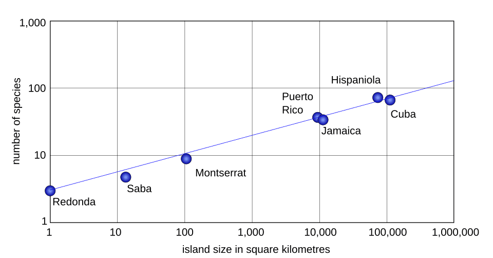
For true oceanic islands and isolated habitat patches — systems in which each area unit represents an independent community with its own colonisation and extinction dynamics — z-values typically fall between 0.20 and 0.35, with a central tendency near 0.25 to 0.30.^{3, 5} Preston's theoretical derivation from the canonical lognormal predicted z approximately equal to 0.262, and MacArthur and Wilson cited a typical range of 0.20 to 0.35 in their 1967 monograph.^{4, 5} For nested samples within a single contiguous region — where successively larger areas are subsets of one another — z-values are consistently lower, typically between 0.12 and 0.18.^{7, 20} The lower z-values in nested samples reflect the fact that nearby areas share many species, so increasing the sampled area adds relatively few new species compared with sampling a truly independent island of equivalent size.

The constant c in the power function is less often discussed but is ecologically meaningful: it reflects the overall species density of the region or taxon in question. A tropical bird fauna will have a much higher c than a boreal mammal fauna, even if the z-values are similar. The value of c is sensitive to the units in which area is measured, so comparisons of c across studies require standardisation of area units.⁷

Harte, Smith, and Storch offered a reinterpretation of the z-value in terms of the self-similarity of species distributions across spatial scales. They demonstrated that if species distributions exhibit a form of scale invariance — that is, if the probability that a species occupies a given fraction of a landscape is consistent across scales — then the power-law SAR emerges as a mathematical consequence, and z captures the degree of spatial aggregation or clustering of species.¹² A higher z indicates greater spatial turnover in species composition (beta diversity), while a lower z indicates more homogeneous distributions.

Typical z-values by sampling context^{5, 7, 20}

Nested versus independent sampling

A crucial distinction in species-area research is whether the areas being compared represent nested subsets of a single contiguous landscape or independent, isolated units such as separate islands. This distinction, formalised by Scheiner in a classification of six types of species-area curves, profoundly affects both the shape of the relationship and its ecological interpretation.⁹

In nested sampling (Scheiner's Type I and Type II curves), an investigator counts species within progressively larger quadrats or concentric rings within a single continuous habitat. Because larger samples are supersets of smaller ones, every species found in a small plot is automatically present in every larger plot that contains it. The resulting curve is a species accumulation curve, and its slope reflects how rapidly new species are encountered as the observer samples more of the same landscape. The z-values for nested curves are typically low (0.12 to 0.18) because spatial autocorrelation ensures that adjacent areas share most of their species.^{7, 9}

In independent sampling (Scheiner's Type IV curve, often called the island species-area relationship or ISAR), each data point represents a separate, isolated area — a different island, a different forest fragment, a different mountaintop — with its own independent ecological community shaped by its own history of colonisation and extinction.^{9, 14} The ISAR typically yields steeper slopes (z approximately 0.25 to 0.35) because larger islands support more species not merely through passive sampling of a shared species pool but through additional ecological mechanisms: larger islands offer greater habitat diversity, support larger population sizes that are less vulnerable to stochastic extinction, and intercept more colonists.^{5, 21}

Matthews and colleagues demonstrated empirically that ISARs and species accumulation curves are not equivalent even when fitted to the same habitat-island system, because the mechanisms generating each pattern differ.¹⁴ The ISAR reflects the combined effects of area on habitat heterogeneity, population viability, and immigration-extinction dynamics, whereas the accumulation curve reflects primarily the spatial structure of species distributions within a continuous landscape. Conflating the two types of curve can lead to erroneous conclusions about the ecological processes responsible for the observed species-area pattern.^{14, 19}

Ecological mechanisms

Several non-mutually exclusive mechanisms have been proposed to explain why larger areas contain more species. The simplest is the passive sampling hypothesis, which holds that larger areas contain more individuals and therefore sample a greater proportion of the regional species pool by chance alone. Under this hypothesis, the SAR is essentially a statistical artefact of abundance: rare species are more likely to be encountered when more individuals are counted.^{7, 21} While passive sampling undoubtedly contributes to observed species-area patterns, particularly in nested mainland surveys, it cannot fully account for the steeper slopes observed on true islands, where area affects not just sampling probability but actual community composition.

The habitat diversity hypothesis proposes that larger areas encompass a greater variety of habitats — different soil types, elevational zones, vegetation structures, microclimates — and that each habitat supports a distinct set of specialist species.⁷ Empirical studies have repeatedly shown that habitat heterogeneity correlates positively with species richness, and that controlling for habitat diversity reduces the apparent effect of area, though it rarely eliminates it entirely.²¹

The area per se hypothesis, central to MacArthur and Wilson's equilibrium theory, holds that area directly affects extinction rates independently of habitat diversity. Larger islands support larger populations, and larger populations are less susceptible to demographic stochasticity, environmental fluctuations, and catastrophic events that can drive small populations to extinction.^{5, 6} The equilibrium theory predicts that larger islands will maintain higher equilibrium species numbers because their per-species extinction rates are lower, even if the rate of immigration is held constant.

Wang and colleagues proposed a synthetic framework for dissecting these mechanisms, demonstrating that the ISAR on real archipelagos typically reflects contributions from all three processes — passive sampling, habitat heterogeneity, and area-dependent extinction — in proportions that vary among taxonomic groups and geographic settings.²¹

Applications in conservation biology

The species-area relationship has become one of the most widely used tools in conservation biology for predicting species losses from habitat destruction.

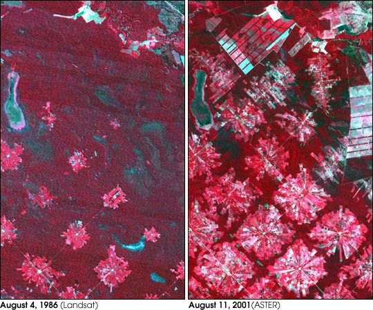
The logic is straightforward: if S = cA^z describes the relationship between species richness and habitat area, then reducing habitat area from A to A′ should reduce equilibrium species richness from S to S′ = cA′^z. The fraction of species predicted to go extinct is therefore 1 − (A′/A)^z. This "reverse species-area curve" approach has been applied to estimate extinction risks from tropical deforestation, wetland drainage, and climate-driven range contraction.^{10, 11}

In a widely cited 2004 study, Thomas and colleagues applied species-area reasoning to project extinction risks under future climate change scenarios. Using distributional data for 1,103 species of plants, mammals, birds, reptiles, frogs, butterflies, and other invertebrates, they estimated that 15 to 37 percent of species in their sample regions would be "committed to extinction" by 2050 under mid-range climate warming scenarios, based on the projected contraction of climatically suitable habitat area.¹¹ The study generated enormous public and scientific attention and helped galvanise concern about climate-driven biodiversity loss.¹⁷

However, subsequent work revealed a fundamental problem with the backward extrapolation. In 2011, He and Hubbell demonstrated that species-area relationships systematically overestimate extinction rates when applied in reverse. The mathematical basis of the problem is a geometric sampling asymmetry: the area required to encounter a species for the first time (the species accumulation process that builds the SAR) is systematically smaller than the area that must be destroyed to eliminate the last individual of that species (the extinction process).¹⁰ Because species are spatially aggregated rather than randomly distributed, destroying a given fraction of habitat removes a smaller fraction of species than the SAR would predict. He and Hubbell showed that the correct backward extinction curve is not the inverse of the forward SAR but a distinct function — the endemics-area relationship (EAR) — which counts only species found exclusively within a given area. The EAR consistently yields lower extinction estimates than the SAR for the same amount of habitat loss.^{10, 16}

This finding does not imply that habitat loss is inconsequential for biodiversity. Species that persist in reduced habitat fragments may face declining population sizes, loss of genetic diversity, disrupted ecological interactions, and elevated vulnerability to future disturbances — a phenomenon known as extinction debt, in which species persist temporarily in a non-equilibrium state before eventually disappearing.¹⁶ Kitzes and Harte proposed improved macroecological methods for estimating extinction that account for the spatial distribution of species and the geometry of habitat loss, yielding more accurate predictions than the simple backward SAR.¹⁸ The lesson for conservation practitioners is that the species-area relationship remains a valuable first-order tool for gauging the consequences of habitat loss, but that its backward application requires careful attention to the distinction between the species encountered in an area and the species endemic to that area.

Ongoing research and synthesis

Despite more than a century of study, the species-area relationship continues to generate active research. One productive area of inquiry concerns the scale dependence of the SAR: the z-exponent is not constant across all spatial scales but instead tends to be low at very small scales (within-habitat sampling), higher at intermediate scales (among islands or habitat patches), and highest at biogeographic scales spanning entire continents or biomes, where evolutionary diversification and historical contingency drive species turnover.^{7, 12} This triphasic pattern, first described by Preston and elaborated by Rosenzweig, suggests that different processes dominate the species-area relationship at different spatial grains.

A second area of active investigation is the search for mechanistic models that can predict the SAR from first principles. Neutral theory, maximum entropy approaches, and spatially explicit simulation models have all been deployed to derive species-area curves from assumptions about dispersal, speciation, and community assembly.^{12, 18} These efforts aim to move beyond the purely descriptive fitting of power functions to an understanding of why the power function works as well as it does and under what conditions it should fail.

Finally, the distinction between ISARs and species accumulation curves, formalised by Scheiner and reinforced by Matthews and colleagues, has prompted more careful attention to the sampling design underlying any claimed species-area relationship.^{9, 14} As ecologists increasingly apply species-area reasoning to habitat islands such as urban parks, agricultural fragments, and mountaintop refugia, the question of whether these systems behave like true islands — with independent colonisation and extinction dynamics — or like nested samples of a continuous landscape has direct consequences for the validity of the resulting predictions.^{19, 21}