Overview
- Isostasy is the principle of gravitational equilibrium between Earth's rigid lithosphere and the underlying ductile asthenosphere, explaining why mountains have deep crustal roots and why continents float at elevations proportional to their thickness and density.
- The concept emerged from 18th- and 19th-century geodetic observations showing that the Andes and Himalayas deflect plumb lines far less than their visible mass would predict, implying compensating mass deficits at depth that balance the topographic load.
- Glacial isostatic adjustment, the slow rebound of land surfaces after ice-sheet removal, provides a direct modern demonstration of isostasy and has been measured at rates exceeding 10 mm/yr in Fennoscandia and Hudson Bay using GPS and the GRACE satellite gravity missions.
Isostasy is the condition of gravitational equilibrium between Earth's lithosphere and the underlying asthenosphere, such that the rigid outer shell of the planet floats at an elevation determined by its thickness and density. The concept is often compared to an iceberg floating in water: just as the proportion of ice above and below the waterline is governed by the relative densities of ice and seawater, so the elevation of a crustal block above or below the datum of the surrounding terrain is governed by the density contrast between the lithosphere and the denser mantle beneath it.4, 13 Mountains stand high not only because material has been piled up at the surface but because their crust extends as a deep root into the mantle, displacing denser material and achieving buoyant support. Conversely, ocean basins are low because their thin, dense oceanic crust sits at a lower equilibrium level than the thicker, less dense continental crust.
The principle of isostasy is fundamental to understanding a wide range of geological phenomena, from the architecture of mountain belts and the subsidence of sedimentary basins to the ongoing rebound of landmasses freed from Pleistocene ice sheets. It was the unexpected behaviour of pendulums and plumb lines near great mountain ranges in the 18th and 19th centuries that first revealed the existence of compensating mass deficits at depth, and the subsequent theoretical frameworks developed by Pratt and Airy remain foundational to geophysics more than 160 years later.1, 2
The geodetic discovery of isostasy
The story of isostasy begins with geodesy, the science of measuring the shape and gravitational field of the Earth. In 1735, the French astronomer Pierre Bouguer joined a geodetic expedition to the equatorial Andes, sponsored by the French Academy of Sciences, to determine the precise figure of the Earth by measuring a degree of latitude near the equator. While in Peru, Bouguer made gravity measurements using a pendulum and observed that the gravitational attraction of the Andes was far weaker than would be expected from the visible mass of the mountains. Specifically, he measured the deflection of a plumb line near the volcano Chimborazo and found it to be only about 7 arc-seconds, compared with the roughly 103 arc-seconds predicted by Newtonian gravity assuming the mountains had uniform rock density throughout.4, 21 Bouguer had no satisfactory explanation for this discrepancy, but his observation that large topographic masses produced a gravity signal much weaker than expected was the first empirical hint that something beneath the mountains was compensating for their mass.
The question resurfaced a century later during the Great Trigonometrical Survey of India, directed by George Everest. Surveyors comparing astronomical latitude measurements (determined by the position of stars relative to the local vertical, defined by a plumb line) with geodetic latitude measurements (determined by triangulation from a baseline) found systematic discrepancies near the Himalayan front. At stations such as Kalianpur in the Indo-Gangetic Plain, the plumb line was deflected toward the Himalayas, as expected from the gravitational attraction of the mountain mass, but the observed deflection was only about one-third of what the visible topography alone would predict.1, 4 This deficiency demanded explanation: somehow the mass excess represented by the Himalayas at the surface was being partially cancelled by a mass deficit at depth.
Two rival explanations were published in 1855. John Henry Pratt, Archdeacon of Calcutta, proposed that the reduced deflection could be explained if the crust beneath mountains were less dense than the crust beneath lowlands, so that all columns of rock standing above some uniform depth of compensation had the same total mass per unit area.1 George Biddell Airy, the Astronomer Royal, proposed instead that the crust everywhere has approximately the same density but varies in thickness, with mountains possessing deep roots that extend into the denser mantle, much as icebergs with tall freeboard have proportionally deeper keels below the waterline.2 Both models predict that the gravitational attraction of surface topography will be partially offset by a compensating mass distribution at depth, and both produce calculated plumb-line deflections much closer to the observed values than an uncompensated model. The term "isostasy" itself was coined in 1889 by the American geologist Clarence Dutton to describe this condition of gravitational balance.3
Airy isostasy and crustal roots
In the Airy model of isostasy, variations in surface elevation are supported by variations in the thickness of a crust of uniform density floating on a denser substratum. The analogy is directly to Archimedes' principle: a block of wood floating in water sinks until the weight of the water it displaces equals its own weight, and a thicker block floats with both a higher freeboard and a deeper draft. In the Airy formulation, mountains are underlain by thick crustal roots that protrude downward into the mantle, while ocean basins have thin crust with correspondingly shallow roots.2, 4
The mathematical expression of Airy isostasy is straightforward. If a mountain of height h above sea level is supported by a crustal root of depth r below some reference depth, and if the crustal density is ρc and the mantle density is ρm, then the equilibrium condition requires that the weight of the root displaced into the mantle equals the weight of the topography above the reference level: r = h · ρc / (ρm − ρc). For typical values of ρc ≈ 2,800 kg/m³ and ρm ≈ 3,300 kg/m³, a 5-kilometre mountain requires a root approximately 28 kilometres deep, meaning that the total crustal thickness beneath a major mountain range is far greater than the standard continental crust thickness of 35 to 40 kilometres.4, 13
Seismological observations have confirmed the Airy prediction that mountain belts are underlain by anomalously thick crust. The Himalaya-Tibet collision zone, the most dramatic example on Earth, has crustal thicknesses reaching 70 to 80 kilometres beneath the Tibetan Plateau, approximately double the global continental average. The Project INDEPTH seismic surveys of southern Tibet revealed not only this extreme crustal thickness but also evidence of a partially molten layer within the middle crust, produced by the enormous pressure and heat generated by continued India-Eurasia convergence.15, 18 Beneath the European Alps, the Andes, and the North American Cordillera, seismic receiver-function studies similarly document crustal roots of 50 to 65 kilometres, consistent with Airy isostatic compensation of the overlying topography.4
Pratt isostasy and lateral density variations
The Pratt model takes a fundamentally different approach. Rather than invoking variations in crustal thickness, it explains topographic variations through lateral differences in crustal density, all above a uniform depth of compensation. In this framework, mountain regions are composed of rock that is less dense than the rock beneath lowlands, and each vertical column of material from the surface down to the compensation depth has the same total mass per unit area. Topographic highs correspond to columns of lower average density, while topographic lows correspond to columns of higher average density.1, 4
Pratt refined his model in subsequent publications, demonstrating more rigorously how lateral density variations could account for the reduced plumb-line deflections observed near the Himalayas. He showed that if the compensation depth were approximately 100 kilometres and the density of the crust varied inversely with its surface elevation, the calculated gravitational deflection matched the geodetic observations far more closely than any uncompensated model.1, 22 In the early 20th century, the American geodesist John Hayford and the Finnish geodesist Veikko Heiskanen formalized and extended the Pratt and Airy models respectively, establishing quantitative frameworks still used in geodetic calculations today. The Pratt-Hayford model proved particularly useful for reducing gravity observations over broad oceanic and continental regions.4
In practice, both Airy and Pratt compensation contribute to the isostatic equilibrium of real geological structures. Mid-ocean ridges, for example, stand elevated above the surrounding abyssal plains primarily because of the Pratt mechanism: the hot, young lithosphere near the ridge axis is less dense than the cold, old lithosphere far from the ridge, and this density contrast drives the topographic variation along a profile of approximately uniform crustal thickness.13 Continental mountain belts, by contrast, are better described by the Airy mechanism, with their thick crustal roots providing the dominant buoyant support. Most real geological settings involve some combination of both effects.4
Flexural isostasy and elastic thickness
The classical Airy and Pratt models treat the lithosphere as if it were composed of independent vertical columns with no lateral mechanical coupling, a condition known as local or pointwise compensation. In reality, the lithosphere has finite mechanical strength and responds to applied loads not as a collection of isolated columns but as a continuous elastic plate that bends and distributes the load over an area much wider than the load itself. This behaviour is described by the theory of flexural isostasy, which was placed on a rigorous quantitative footing by the work of A. B. Watts and colleagues from the 1970s onward.4, 5
The central parameter in flexural isostasy is the effective elastic thickness (Te) of the lithosphere, which is a measure of its long-term mechanical rigidity under geological loads. Te is not the physical thickness of any single layer but an integrated measure of the plate's resistance to bending. A lithosphere with a large Te is stiff, distributes loads broadly, and deflects gently over a wide area; a lithosphere with a small Te is weak and deflects sharply beneath the load, approaching the Airy limit of local compensation.4, 7
In the oceans, Watts demonstrated that Te increases systematically with the square root of the age of the oceanic lithosphere at the time of loading, reflecting the progressive cooling and thickening of the lithospheric thermal boundary layer. His seminal 1978 study of the Hawaiian-Emperor Seamount Chain showed that the best-fitting Te values were 20 to 30 kilometres, corresponding to the depth of the roughly 300–600°C isotherm in the cooling oceanic plate.5, 20 Continental lithosphere is more complex, with Te values ranging from less than 5 kilometres in hot, tectonically active regions to more than 80 kilometres in cold, stable cratons, reflecting the strong dependence of lithospheric rheology on temperature, composition, and tectonic history.7
The spectral methods used to estimate Te from gravity and topography data were refined by Forsyth, who showed that both surface and subsurface loading must be considered when interpreting the coherence between Bouguer gravity anomalies and topography.6 These methods have since been applied globally, producing maps of Te that reveal fundamental differences in lithospheric strength between tectonic provinces and provide constraints on the thermal and compositional structure of the lithosphere that are complementary to those derived from seismology.4, 7
Effective elastic thickness (Te) by tectonic setting4, 5, 7
| Tectonic setting | Typical Te (km) | Controlling factors |
|---|---|---|
| Young oceanic (<25 Ma) | 2–15 | Thin thermal lithosphere, high heat flow |
| Old oceanic (>80 Ma) | 25–50 | Thick, cold thermal lithosphere |
| Continental rift zones | 5–15 | Elevated geotherm, thinned lithosphere |
| Active orogens | 15–40 | Thick crust, moderate geotherm |
| Stable continental shields | 40–100+ | Cold, thick, depleted cratonic lithosphere |
Free-air and Bouguer gravity anomalies

.jpg)
The state of isostatic compensation of a region is assessed through gravity anomalies, which are the differences between observed gravitational acceleration and the value predicted by a theoretical reference model. Two types of anomaly are particularly important in isostatic studies. The free-air anomaly corrects the observed gravity for the elevation of the measurement station above the reference ellipsoid but does not account for the gravitational attraction of the rock mass between the station and the ellipsoid. The Bouguer anomaly applies an additional correction for the gravitational effect of this intervening rock mass, approximated as an infinite slab of specified density (the Bouguer correction) and, in more refined analyses, for the irregularities of the surrounding terrain (the terrain correction).4, 21
Over isostatically compensated topography, the free-air anomaly is close to zero, because the mass of the topographic load at the surface is exactly offset by the mass deficit of the compensating root at depth. The Bouguer anomaly, by contrast, is strongly negative over mountains and positive over ocean basins, because the Bouguer correction removes the effect of the surface topography but not the effect of the compensating root, which represents a genuine mass deficit relative to the surrounding mantle. A large Bouguer anomaly of −400 to −500 milligals over the Tibetan Plateau, for example, reflects the enormous crustal root extending to 70 or more kilometres depth beneath the plateau.4, 15
Free-air anomalies that deviate significantly from zero indicate regions that are not in isostatic equilibrium. Positive free-air anomalies over a topographic feature suggest that the feature is supported at least partly by the mechanical strength of the lithosphere rather than by a compensating root, a condition typical of loads smaller than the flexural wavelength of the plate. Negative free-air anomalies can indicate areas of active subsidence or dynamic topography maintained by viscous stresses in the convecting mantle rather than by isostatic buoyancy.4, 13
The geoid, the equipotential surface of Earth's gravity field that corresponds to mean sea level over the oceans, provides another window into isostatic compensation. Undulations in the geoid reflect the distribution of mass anomalies within the Earth, with positive geoid heights corresponding to mass excesses and negative geoid heights to mass deficits. Satellite missions such as GRACE (Gravity Recovery and Climate Experiment) and its successor GRACE-FO have mapped the geoid with unprecedented precision, enabling the detection of gravity changes on monthly timescales associated with ice-sheet mass loss, groundwater depletion, and the ongoing viscous response of the mantle to deglaciation.19
Glacial isostatic adjustment
The most dramatic modern demonstration of isostasy in action is glacial isostatic adjustment (GIA), the ongoing response of the solid Earth to the growth and decay of the great Pleistocene ice sheets. During the Last Glacial Maximum, approximately 26,000 to 19,000 years ago, ice sheets several kilometres thick covered northern Europe, northern North America, and parts of Siberia. Their immense weight depressed the underlying lithosphere by hundreds of metres, displacing mantle material laterally and raising a peripheral bulge around the margins of the ice sheets. When the ice melted, the load was removed, but the viscous mantle could not flow back instantaneously; instead, the depressed regions began to rebound slowly, a process that continues to this day thousands of years after the ice disappeared.8, 17
The earliest scientific recognition that Scandinavia was rising came from observations of old shorelines stranded above present sea level along the coasts of Sweden and Finland. By the early 20th century, tide-gauge records spanning decades confirmed that the land was rising at measurable rates. The Norwegian explorer and scientist Fridtjof Nansen published an influential synthesis in 1928 linking this uplift to the removal of the glacial load, and Norman Haskell in 1935 used the Fennoscandian uplift data to derive the first quantitative estimate of the viscosity of Earth's mantle, obtaining a value of approximately 1021 pascal-seconds that has proved remarkably durable.16, 17
Modern GPS networks have transformed the measurement of GIA from a historical reconstruction into a real-time observation. The BIFROST (Baseline Inferences for Fennoscandian Rebound Observations, Sea Level, and Tectonics) project, which has operated a network of continuously recording GPS receivers across Sweden and Finland since the 1990s, has documented present-day vertical uplift rates reaching approximately 10 mm/yr in the northern Gulf of Bothnia, the region that was beneath the thickest part of the Fennoscandian ice sheet.9, 10 Uplift rates decrease radially outward from this centre and transition to subsidence of 1 to 2 mm/yr in areas that were on the peripheral bulge, such as the coasts of the Netherlands and northern Germany, where the bulge is now collapsing as mantle material flows back toward the rebounding centre.10, 12
In North America, a similar pattern is observed. GPS measurements from more than 360 sites across Canada and the United States show present-day uplift of approximately 10 mm/yr near Hudson Bay, the former centre of the Laurentide Ice Sheet, with rates decreasing outward and transitioning to peripheral subsidence of 1 to 2 mm/yr south of the Great Lakes.11 The GRACE and GRACE-FO satellite gravity missions have independently confirmed these patterns by detecting the increase in gravitational attraction over rebounding regions as mantle material flows back beneath them, providing a powerful complement to the GPS measurements of surface deformation.19, 24
Present-day vertical uplift rates from glacial isostatic adjustment9, 10, 11
GIA modelling and mantle viscosity
Glacial isostatic adjustment serves as one of the most powerful natural experiments for constraining the viscosity structure of Earth's mantle. Because the timescale and spatial pattern of the rebound depend on how readily mantle material flows in response to the removal of the ice load, observations of uplift rates, relative sea-level histories, and gravity changes can be inverted to infer the viscosity of the mantle at different depths. This approach has yielded one of the most robust geophysical constraints on the deep Earth: an upper-mantle viscosity of approximately 3–5 × 10²⁰ pascal-seconds and a lower-mantle viscosity one to two orders of magnitude higher, in the range of 1021 to 1022 pascal-seconds.8, 12, 16
The most widely used GIA models combine a detailed reconstruction of the history of ice loading and unloading with a model of the Earth's viscoelastic response. The ICE-5G (VM2) model developed by W. R. Peltier specifies the spatial extent and thickness of the global ice sheets at intervals through the last glacial cycle, coupled to a radially stratified mantle viscosity profile. This model has been calibrated against relative sea-level records from formerly glaciated and peripheral regions, GPS-measured uplift rates, and, more recently, the time-variable gravity field observed by the GRACE satellite mission.8 The availability of GRACE data has been particularly transformative, because the gravity changes associated with GIA provide a constraint on mantle flow that is independent of, and complementary to, the constraints from surface deformation and sea-level records.19
GIA modelling also has important practical applications. Accurate predictions of the ongoing rebound are essential for interpreting tide-gauge records of sea-level change, because the apparent rate of sea-level rise or fall at a given coastal station is the sum of the actual change in ocean volume and the vertical motion of the land on which the gauge sits. In regions of strong post-glacial rebound, such as the northern Baltic Sea, relative sea level is actually falling despite the global rise in ocean volume, while on the peripheral bulge, the subsidence of the land amplifies the apparent rate of sea-level rise.12, 23 The correct separation of the GIA signal from the mass-change signal is also critical for using GRACE data to monitor ice-sheet mass balance and groundwater storage, since the gravitational signature of ongoing mantle flow overlaps spatially with the signals of interest.19, 24
Isostasy and mountain building
The principle of isostasy is central to understanding the growth, support, and eventual collapse of mountain belts. When two continental plates collide, the crust between them is shortened and thickened by folding, faulting, and ductile flow. As the crust thickens, it sinks deeper into the mantle in accordance with Airy isostasy, developing a root that provides buoyant support for the growing mountain range. The Himalaya-Karakoram-Tibet system, produced by the collision of the Indian and Eurasian plates beginning approximately 50 million years ago, exemplifies this process on a grand scale. The collision has doubled the normal continental crustal thickness over an area of more than 5 million square kilometres, creating the Tibetan Plateau at an average elevation of roughly 5,000 metres above sea level, supported by a crustal root extending to 70–80 kilometres depth.15, 18
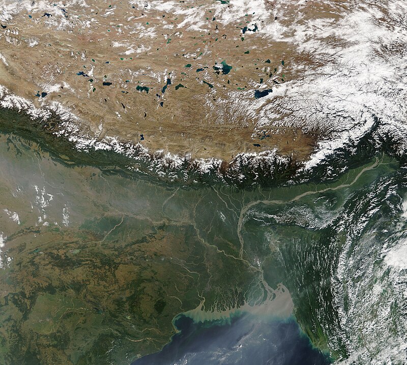
.jpg)
Isostasy also governs the feedback between erosion and uplift that shapes mountain belts over geological time. As erosion removes mass from the surface of a mountain range, isostatic equilibrium demands that the lightened crust rebound upward to partially restore the topographic relief. This isostatic response to erosion means that mountains can maintain substantial elevations long after the tectonic forces that built them have ceased, because the removal of each increment of surface rock brings deeper, previously buried rock upward. The net result is that a mountain range must erode away a total mass much greater than its initial topographic relief before it is finally reduced to a peneplain.4, 13
At the other extreme, the loading of the lithosphere by volcanic or sedimentary material produces a flexural depression whose geometry depends on the effective elastic thickness. The weight of the Hawaiian volcanic chain, for example, has depressed the Pacific plate into a broad moat around the islands, with an arch of slight uplift beyond the moat where the plate flexes upward in response to the bending. Watts' analysis of the gravity and bathymetry across the Hawaiian-Emperor chain provided one of the earliest and clearest demonstrations that the lithosphere responds to loads as an elastic plate rather than as a set of independent columns.5
Isostasy, rift basins, and sea-level change
Isostatic principles govern the formation and evolution of sedimentary basins, which are regions where the lithosphere subsides and accommodates thick accumulations of sediment. The most influential model of rift-basin formation, developed by Dan McKenzie in 1978, treats the lithosphere as an elastic plate that is uniformly stretched and thinned during a rifting event. The thinning reduces both the crustal thickness (which lowers the surface through Airy isostasy) and the lithospheric thermal structure (which initiates a phase of thermal contraction and further subsidence as the stretched lithosphere cools back to equilibrium).14 The McKenzie model predicts a two-stage subsidence history: an initial rapid syn-rift phase driven by mechanical thinning, followed by a prolonged post-rift phase of slower, thermally driven subsidence. This two-stage pattern has been observed in rift basins worldwide, including the North Sea, the Gulf of Suez, and the passive margins of the Atlantic Ocean.13, 14
On a global scale, isostasy links the solid Earth to sea-level change through several pathways. The growth of ice sheets during glacial periods depresses the land beneath them and draws water from the oceans, lowering global sea level. But the reduction in ocean mass also unloads the ocean basins, which rebound upward, partially offsetting the sea-level fall. Conversely, when ice melts and the water returns to the oceans, the ocean floor is depressed by the additional load while the formerly glaciated regions rebound upward. These effects produce a geographically variable pattern of sea-level change called a sea-level fingerprint, in which the magnitude and even the sign of sea-level change differs from location to location depending on the pattern of ice loading and the viscoelastic response of the Earth.23
Understanding these isostatic contributions to sea-level change is critical for interpreting both the geological record of past sea levels and modern observations of sea-level rise. Tide-gauge records, satellite altimetry, and GRACE gravity measurements must all be corrected for the ongoing effects of glacial isostatic adjustment before they can yield reliable estimates of the contribution of present-day ice-sheet mass loss to global sea-level rise. The uncertainty in the GIA correction remains one of the largest sources of error in estimates of Antarctic and Greenland ice-sheet mass balance derived from satellite gravity data.19, 24
References
On the attraction of the Himalaya Mountains, and of the elevated regions beyond them, upon the plumb-line in India
On the computation of the effect of the attraction of mountain-masses, as disturbing the apparent astronomical latitude of stations in geodetic surveys
Lithospheric strength and its relationship to the elastic and seismogenic layer thickness
Global glacial isostasy and the surface of the ice-age Earth: the ICE-5G (VM2) model and GRACE
Continuous GPS measurements of postglacial adjustment in Fennoscandia: 1. Geodetic results
An improved and extended GPS-derived 3D velocity field of the glacial isostatic adjustment (GIA) in Fennoscandia
Partially molten middle crust beneath southern Tibet: synthesis of Project INDEPTH results
Glacial isostatic adjustment modelling: historical perspectives, recent advances, and future directions
On the deflection of the plumb-line in India caused by the attraction of the Himalaya mountains and the elevated regions beyond, and its modification by the compensating effect of a deficiency of matter below the mountain mass
The moving boundaries of sea level change: understanding the origins of geographic variability
Continuity of ice sheet mass loss in Greenland and Antarctica from the GRACE and GRACE Follow-On missions