Overview
- Stars are sorted by surface temperature into the OBAFGKM sequence—from blue-hot O stars above 30,000 K down to red M dwarfs below 3,500 K—with each class revealing distinct absorption lines, masses, and lifespans.
- The Morgan–Keenan luminosity system adds a Roman numeral (I through V) to distinguish supergiants from giants from main-sequence dwarfs, so a single two-part label like G2 V fully locates a star on the Hertzsprung-Russell diagram.
- Classification underpins virtually every branch of modern astrophysics, from calibrating the cosmic distance ladder to tracing the chemical evolution of galaxies across stellar populations.
When astronomers direct a spectrograph at a star and spread its light into a rainbow of wavelengths, they find the spectrum is not continuous. Dark absorption lines interrupt it at precise positions—each line corresponding to a specific element whose atoms in the stellar atmosphere have absorbed that wavelength of radiation. The pattern of these lines is so distinctive and reproducible that it encodes, in a single measurement, a star’s surface temperature, its gravity, its chemical composition, and its evolutionary state. Stellar classification is the formal system that extracts this information and organizes stars into a coherent taxonomy. It is among the most powerful acts of scientific compression ever achieved: a few characters of shorthand that locate any star in a space defined by physics, chemistry, and cosmological history.1, 2
The system used today is the product of two distinct efforts. The Harvard spectral classification, developed at the close of the nineteenth century and refined in the early twentieth, sorted stars by temperature using their absorption-line patterns. The Morgan–Keenan (MK) luminosity system, introduced in 1943, added a second dimension to distinguish stars of the same temperature but vastly different sizes and luminosities. Together, these two components map directly onto the Hertzsprung-Russell diagram, the fundamental organizational tool of stellar astronomy, and form the backbone of our understanding of stellar evolution.2, 5
The Harvard spectral classification
In the 1880s, the director of the Harvard College Observatory, Edward Pickering, launched an ambitious survey of stellar spectra. A team of women astronomers—known today as the Harvard Computers—catalogued the spectra of hundreds of thousands of stars. Williamina Fleming introduced an alphabetical scheme running from A through Q based on the strength of hydrogen absorption lines. Annie Jump Cannon subsequently reorganized and greatly simplified the system, collapsing it to the letters that remain in use: O, B, A, F, G, K, M. Cannon’s insight was that the spectral sequence is primarily a temperature sequence, not a hydrogen-line sequence, and that rearranging the letters into temperature order produced a logically unified picture.4
The resulting sequence runs from hottest to coolest, and the traditional mnemonic for memorizing it—Oh Be A Fine Girl/Guy, Kiss Me—has been passed between generations of astronomy students since the early twentieth century.1 Each letter designates a class, and each class is further subdivided by a numeral from 0 to 9, where 0 is hotter and 9 is cooler within that class. The Sun, for instance, falls at G2, placing it in the hotter portion of the G class. This numerical subdivision was formalized in the MK system and allows fine discrimination between closely similar stars.2, 3
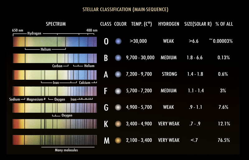
Harvard spectral classes: temperature, color, and example stars1, 2, 6
| Class | Temperature (K) | Color | Dominant spectral lines | Example |
|---|---|---|---|---|
| O | >30,000 | Blue | Ionized helium (He II) | Naos (ζ Puppis) |
| B | 10,000–30,000 | Blue-white | Neutral helium (He I), hydrogen | Rigel |
| A | 7,500–10,000 | White | Hydrogen (Balmer series, strongest) | Sirius |
| F | 6,000–7,500 | Yellow-white | Ionized calcium (Ca II), hydrogen weakening | Procyon |
| G | 5,200–6,000 | Yellow | Ca II H & K lines strongest, metal lines | The Sun |
| K | 3,700–5,200 | Orange | Metal lines, molecular CH bands | Arcturus |
| M | 2,400–3,700 | Red | Titanium oxide (TiO) molecular bands | Proxima Centauri |
The physical basis: temperature and absorption lines
The absorption lines that define each spectral class arise from a straightforward piece of atomic physics. When photons from a stellar interior pass through the cooler gas of a stellar atmosphere, atoms absorb photons at energies corresponding to specific electronic transitions. The pattern of which transitions occur—and therefore which lines appear—depends critically on temperature, because temperature governs which energy levels are populated and what fraction of the gas is ionized.6
In O stars, temperatures above 30,000 K are sufficient to strip one electron from helium, producing singly ionized helium (He II). These ions dominate the spectrum. Hydrogen is present but much of it is fully ionized, so its Balmer absorption lines are paradoxically weak. In A stars, where temperatures hover around 9,000 K, hydrogen is in its optimal excitation state for Balmer absorption—the second energy level is thermally populated without being ionized—so hydrogen lines reach their maximum strength. Moving into the cooler F, G, and K classes, the gas is cool enough for calcium to survive in singly ionized form (Ca II), and the famous H and K lines of ionized calcium dominate the optical spectrum. In the M class, temperatures fall below about 3,500 K, low enough for simple molecules to form: titanium oxide and vanadium oxide produce characteristic broad molecular absorption bands that give M stars their red color and distinguish them immediately from hotter types.6, 2
This temperature sequence is a direct consequence of stellar physics. A star’s surface temperature is determined primarily by its mass: more massive stars contract to higher core temperatures and higher luminosities, and they radiate from hotter surfaces. The spectral type is therefore a proxy for mass on the main sequence, a relationship that becomes quantitatively precise through the mass-luminosity relation.6, 13
The Morgan–Keenan luminosity classes
By the 1940s it was well established that two stars could share the same spectral type—the same surface temperature and the same absorption-line pattern—while differing enormously in intrinsic luminosity. A cool red star might be a faint M-class dwarf like Proxima Centauri, 10,000 times less luminous than the Sun, or it might be a red supergiant like Betelgeuse, 100,000 times more luminous. Temperature alone cannot distinguish them. The physical reason is that luminosity depends on both temperature and the total radiating surface area: L = 4πR²σT4, where a dramatically larger radius more than compensates for modest temperature differences.2, 3
William Wilson Morgan, Philip Keenan, and Edith Kellman addressed this in their 1943 Atlas of Stellar Spectra, which defined the MK luminosity classes. They noticed that subtle differences in spectral line width and line ratio could discriminate luminosity at fixed temperature. In giant and supergiant stars, the lower atmospheric pressure (a consequence of their lower surface gravity) produces narrower, sharper spectral lines than in the denser atmospheres of dwarfs. Certain line ratios between adjacent ionization states of the same element are exquisitely sensitive to gravity. Using these diagnostics, Morgan and Keenan defined five luminosity classes designated by Roman numerals:2, 3
Class I designates supergiants, further divided into Ia (most luminous) and Ib (less luminous). These are the most massive, most luminous, and shortest-lived evolved stars. Class II identifies bright giants, occupying a region between supergiants and normal giants on the Hertzsprung-Russell diagram. Class III encompasses ordinary giants, stars that have evolved off the main sequence and expanded as they exhaust their core hydrogen. Class IV labels subgiants, stars beginning to evolve away from the main sequence but not yet fully expanded. Class V designates the main sequence—also called dwarfs—where stars spend the majority of their lives fusing hydrogen in hydrostatic equilibrium.2, 3
The full MK classification combines spectral type and luminosity class into a single compact label. The Sun is G2 V: spectral type G, subclass 2, luminosity class V (main-sequence dwarf). Rigel is B8 Ia: a hot, blue, extremely luminous supergiant. Arcturus is K1.5 III: a cool orange giant. This two-part label places any star precisely on the HR diagram and, by extension, into its evolutionary narrative.1, 3
Spectral classes in detail
O stars are the rarest and most extreme objects on the main sequence, comprising less than one star in a million in the solar neighborhood.15 Their masses range from roughly 16 to over 100 solar masses, their luminosities from 30,000 to more than one million times that of the Sun, and their surface temperatures from 30,000 to above 50,000 K. They burn through their hydrogen fuel in as little as a few million years—a cosmic eyeblink compared to the Sun’s 10-billion-year main-sequence lifetime. The prototype of extreme O stars is Naos (ζ Puppis), an O4 If supergiant so luminous that it ionizes vast volumes of the surrounding interstellar gas. O stars are the primary ionizing agents of H II regions, the glowing nebulae that mark recent star formation.15, 6
B stars include some of the sky’s most familiar and brilliant objects. Their temperatures from 10,000 to 30,000 K produce neutral helium lines alongside strong hydrogen lines. Rigel (B8 Ia) in Orion is a blue supergiant shining at roughly 120,000 solar luminosities, detectable to the naked eye across 860 light-years. Spica (α Virginis) is a close B-star binary. Achernar (α Eridani), one of the most rapidly rotating stars known, spins fast enough to have flattened into a notably oblate shape. B stars live tens to hundreds of millions of years and typically end their lives as neutron stars after a core-collapse supernova.6
A stars are defined by the maximum strength of the hydrogen Balmer series, which peaks near 9,000 K. Sirius (A1 V), the brightest star in the night sky, is an A star located just 8.6 light-years away. Its apparent brilliance reflects both its intrinsic luminosity—about 25 times the Sun’s—and its proximity. Vega (A0 V) served for decades as the photometric standard against which the brightness of all other stars was measured. A stars have main-sequence lifetimes on the order of one to two billion years.6
F stars straddle the boundary where hydrogen lines weaken and metal lines grow prominent. Procyon (F5 IV–V) in Canis Minor is the nearest F-type star system at 11.5 light-years. F stars are of particular interest in the search for habitable planets: their habitable zones lie at comfortable distances, they are long-lived relative to their more massive counterparts, and their ultraviolet output is moderate enough to avoid rapidly stripping planetary atmospheres. The Sun’s nearest stellar neighbor with a well-characterized planetary system, τ Ceti, is a G-type star (G8.5 V), slightly cooler and less massive than the Sun.6
G stars are yellow-white stars in whose atmospheres ionized calcium dominates the optical spectrum. The Sun (G2 V) is the defining example. G dwarfs have masses between about 0.8 and 1.2 solar masses and main-sequence lifetimes of eight to twelve billion years. Their surface temperatures of roughly 5,200 to 6,000 K produce the yellow-white light most favorable for photosynthesis as it evolved on Earth. Because G stars are long-lived and common, they are prime targets in exoplanet surveys focused on habitability.6, 13
K stars are orange dwarfs cooler than the Sun, with surface temperatures from roughly 3,700 to 5,200 K. Their spectra are dominated by a forest of metal absorption lines and begin to show molecular bands. Arcturus (K1.5 III), the brightest star in the northern sky, is a K giant that has evolved off the main sequence and expanded to roughly 25 solar radii. K dwarfs on the main sequence are regarded by some astrobiologists as potentially superior hosts for life-bearing planets compared to G stars: they are slightly cooler and longer-lived, their habitable zones are well-separated from the star, and their flare activity is lower than in M dwarfs.6
M stars are the most numerous stars in the galaxy, comprising roughly 70 to 75 percent of all stars in the solar neighborhood.13 Their cool surfaces, below about 3,700 K, allow titanium oxide and other molecules to persist, producing the characteristic broad molecular bands in their red spectra. M dwarfs are dim—the faintest have luminosities less than 0.01 percent of the Sun’s—but their extraordinary longevity (trillions of years on the main sequence for the least massive) makes them by far the most common stellar type. Proxima Centauri (M5.5 Ve), the closest known star to the Sun at 4.24 light-years, is a prototypical M dwarf. M supergiants like Betelgeuse (α Orionis) occupy the opposite extreme: cool but enormously luminous evolved stars whose radii, if placed at the Sun, would engulf the inner solar system out to roughly the orbit of Jupiter.6, 13
Extended classes: L, T, Y, and Wolf-Rayet stars
The infrared sky surveys of the late twentieth century, particularly the Two Micron All Sky Survey (2MASS) and the Sloan Digital Sky Survey, revealed large numbers of objects cooler than any classical M star. These demanded new spectral classes beyond the traditional sequence. Three letters were added to accommodate them: L, T, and Y, in order of decreasing temperature, covering the regime of brown dwarfs and the very coolest stellar objects.7, 8, 9
L dwarfs, defined by Kirkpatrick and colleagues in 1999, span temperatures from roughly 1,300 to 2,400 K. Their spectra show metal hydrides (CaH, FeH) and alkali metal lines (sodium, potassium) replacing the titanium oxide bands of M stars, which condense out into dust clouds below about 2,000 K. L dwarfs include both the very lowest-mass hydrogen-burning stars and the most massive brown dwarfs.7 T dwarfs, whose defining feature is the appearance of methane absorption bands in the near-infrared, occupy the temperature range from roughly 700 to 1,300 K. Methane is quickly destroyed at the temperatures typical of stellar photospheres, so its presence signals a truly substellar object incapable of sustained hydrogen fusion.8 Y dwarfs, discovered in 2011 from data collected by NASA’s Wide-field Infrared Survey Explorer (WISE), are the coldest category of all, with effective temperatures below about 700 K—cooler than a kitchen oven. Water vapor and ammonia dominate their spectra. The coolest confirmed Y dwarfs approach room temperature, blurring the conceptual boundary between the coldest brown dwarfs and the warmest gas-giant planets.9
At the opposite temperature extreme, the classical OBAFGKM sequence also fails to capture one important class of extreme objects: Wolf-Rayet stars. These are massive, highly evolved stars that have shed their outer hydrogen envelopes through fierce stellar winds, exposing their hot, helium-burning interiors. Their surface temperatures can exceed 100,000 K—far beyond the O-star range—and their spectra are dominated not by absorption lines but by broad emission lines of helium, carbon, nitrogen, or oxygen, depending on subtype. Wolf-Rayet stars are designated by the prefix WR, followed by a subtype letter: WN (nitrogen-dominated), WC (carbon-dominated), or WO (oxygen-dominated). They represent a brief but crucial phase in the life of the most massive stars, immediately preceding a core-collapse supernova that may produce a neutron star or black hole.10
The mass-luminosity relation
The mass-luminosity relation is one of the most fundamental results in stellar physics. For main-sequence stars, luminosity scales approximately as the fourth power of mass: L ∝ M4 for stars near the mass of the Sun, though the exponent varies somewhat across the full mass range.6, 13 This steep dependence has profound consequences. A star twice as massive as the Sun is not merely twice as luminous but roughly sixteen times more luminous; a star ten times as massive burns at about 10,000 times the solar luminosity. Because the nuclear fuel available is proportional to mass while the rate of consumption scales with luminosity, the main-sequence lifetime is roughly proportional to M/L ∝ M−3. This is why O stars exhaust their hydrogen in a few million years while M dwarfs can remain on the main sequence for trillions of years—far longer than the present age of the universe.6, 13
Below about 0.08 solar masses, the mass is insufficient to sustain stable hydrogen fusion: the core never reaches the approximately 10 million kelvin threshold needed for proton–proton chain reactions to proceed at a rate sufficient to halt gravitational contraction. Objects in this substellar regime are the brown dwarfs classified as late-M, L, T, and Y types. They are not stars in the classical sense, though the most massive of them fuse deuterium briefly during their youth before cooling monotonically toward planetary temperatures over billions of years.13, 7 At the upper mass limit, stars above roughly 150 solar masses become so luminous that radiation pressure destabilizes their outer layers, imposing an upper mass boundary sometimes called the Eddington limit.10
Stellar populations and chemical evolution
In 1944, Walter Baade resolved the bulge of the Andromeda Galaxy into individual stars for the first time using the 100-inch Hooker Telescope, and noticed that the stars he resolved were systematically redder and older-looking than the blue stars of the disk. He formalized this observation into a distinction between two populations: Population I stars, the younger, metal-rich stars found in the disks and spiral arms of galaxies, and Population II stars, the old, metal-poor stars concentrated in galactic bulges, halos, and globular clusters.11
The terms “metal-rich” and “metal-poor” in astronomical usage refer to elements heavier than helium, which astronomers collectively call metals regardless of their chemical properties. Population I stars like the Sun contain roughly 2 percent of their mass in metals, built up over billions of years of chemical enrichment as successive generations of stars have synthesized heavy elements and returned them to the interstellar medium through winds and supernovae. Population II stars, formed early in galactic history before much enrichment had occurred, contain ten to a thousand times less metal. The most extreme members, called extremely metal-poor or ultra metal-poor stars, have iron abundances less than one hundred-thousandth of the solar value, preserving an almost pristine record of the early universe’s chemical state.11, 12
A third category, Population III, designates the hypothetical first generation of stars that formed from the primordial gas left by Big Bang nucleosynthesis—a mixture of approximately 75 percent hydrogen and 25 percent helium with virtually no heavier elements. Without metals, which act as coolants in collapsing gas clouds, Population III stars are thought to have been extremely massive, potentially hundreds of solar masses, and consequently very short-lived. No confirmed Population III star has ever been observed directly, because any star massive enough to have formed from metal-free gas would have exhausted its fuel and exploded billions of years ago. Their existence is inferred from theoretical models of early universe star formation and from the abundance patterns seen in the most metal-poor Population II stars, which bear the nucleosynthetic imprint of the supernovae that ended Population III lives.12
Why classification matters
Stellar classification is not a taxonomic exercise performed for its own sake. It is the entry point into virtually every quantitative application of stellar astronomy. When a spectral type and luminosity class are assigned to a star, they immediately constrain its effective temperature, surface gravity, radius, mass, luminosity, and evolutionary state—a cascade of physical information from two characters of shorthand. This makes classification indispensable to the cosmic distance ladder.14
The technique of spectroscopic parallax illustrates this directly. By classifying a star and reading its absolute magnitude from the MK calibration—the known intrinsic luminosity of each spectral type and luminosity class combination—astronomers can compare that intrinsic brightness to the observed apparent brightness to calculate the distance via the inverse-square law of light. Without spectral classification, no such comparison would be possible. This method extends distance measurements far beyond the reach of geometric parallax, which is limited to a few thousand light-years even with the most precise modern instruments.14, 5
Classification also anchors the study of stellar populations and galactic chemical evolution. By assigning spectral types to large samples of stars and measuring their metallicities from spectral line strengths, astronomers trace the history of heavy element production across cosmic time. The youngest Population I stars in the disk are metal-rich because they formed from gas already enriched by many prior stellar generations. The oldest Population II stars in globular clusters are metal-poor because they formed when the galaxy was young and few prior supernovae had contributed their heavy elements to the interstellar pool. This metallicity gradient across stellar populations is one of the primary observational handles on the rate and history of stellar evolution at a galactic scale.11, 12
In the study of exoplanets, stellar classification determines the physical environment in which planets orbit. The habitable zone—the range of orbital distances at which liquid water could exist on a planetary surface—scales with the host star’s luminosity and therefore with its spectral class. A planet at Earth’s orbital distance around an M dwarf would be frozen; the same planet around an O star would be sterilized by ultraviolet radiation. Knowing a star’s type is the first step in evaluating any planetary system’s potential for life. Classification began as an act of organization, but it became a tool for asking the universe’s deepest questions.6, 13
References
Dwarfs cooler than M: the definition of spectral type L using discoveries from the 2 Micron All Sky Survey (2MASS)
The discovery of Y dwarfs using data from the Wide-field Infrared Survey Explorer (WISE)
A measurement of the cosmic distance scale from type Ia supernovae and stellar distance indicators