Overview
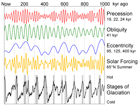
- Three periodic variations in Earth's orbit and axial geometry — eccentricity (~100 ka and ~400 ka), obliquity (~41 ka), and precession (~23 ka and ~19 ka) — redistribute solar energy across latitude and season, pacing the glacial-interglacial cycles of the Quaternary ice age.
- The landmark 1976 study by Hays, Imbrie, and Shackleton demonstrated that the dominant periodicities in deep-sea oxygen isotope records match the calculated orbital frequencies, establishing the astronomical theory of ice ages on firm empirical ground.
- The 100,000-year problem — the dominance of eccentricity-period cycles in the late Pleistocene despite the weakness of eccentricity forcing — and the mid-Pleistocene transition from 41 ka to 100 ka cyclicity remain central unsolved questions in paleoclimatology.
The idea that slow, predictable changes in Earth's orbit around the Sun might govern the advance and retreat of ice sheets is one of the most consequential insights in the earth sciences. Developed in its modern form by the Serbian mathematician and geophysicist Milutin Milankovitch during the first half of the twentieth century, the astronomical theory of ice ages connects celestial mechanics to the geological record of glaciation through three orbital parameters — eccentricity, obliquity, and precession — each operating on a distinct timescale. The theory was confirmed decisively in 1976 when spectral analysis of deep-sea sediment records revealed the precise orbital frequencies that Milankovitch had predicted, and it has since become the foundational framework for understanding Quaternary climate change.1, 3
Milankovitch and the astronomical theory
The notion that astronomical factors might influence Earth's climate predates Milankovitch by nearly a century. In the 1840s, the French mathematician Joseph Adhémar proposed that the precession of the equinoxes could explain ice ages by lengthening winter in one hemisphere. In the 1860s and 1870s, the Scottish scientist James Croll developed a more sophisticated version of the idea, arguing that changes in orbital eccentricity modulated the climatic effect of precession and that ice ages occurred when winter was long and cold in one hemisphere. Croll's theory attracted considerable attention but ultimately fell from favour because the geological dating available at the time appeared to contradict his predicted chronology.3
Milutin Milankovitch, working at the University of Belgrade from the 1910s through the 1940s, revived and transformed the astronomical theory by approaching it as a problem of mathematical physics rather than qualitative reasoning. His central innovation was to calculate, for each latitude and each season, the precise amount of solar radiation (insolation) that Earth's surface would receive given any combination of orbital parameters. This required solving the equations of celestial mechanics for the three relevant orbital variations and then integrating the resulting insolation across the globe. Milankovitch published his comprehensive results in the 1941 monograph Kanon der Erdbestrahlung und seine Anwendung auf das Eiszeitenproblem (Canon of Insolation and the Ice-Age Problem), which included detailed insolation curves for the past 600,000 years at latitudes from the equator to the pole.2
Milankovitch's key insight, following a suggestion by the climatologist Wladimir Köppen, was that the critical factor for ice-sheet growth is not cold winters but cool summers. If summer insolation at high northern latitudes falls below a threshold, winter snowfall fails to melt completely, and the accumulated residue grows year by year into a continental ice sheet. The theory therefore predicts that glacial inception should correlate with minima in Northern Hemisphere summer insolation — a prediction that has been broadly confirmed by the geological record.2, 4
Eccentricity
The first of the three orbital parameters is eccentricity, which describes how much Earth's orbit departs from a perfect circle. A circular orbit has an eccentricity of zero; a highly elongated ellipse approaches an eccentricity of one. Earth's orbital eccentricity varies between approximately 0.005 (nearly circular) and 0.058 (modestly elliptical), driven by the gravitational perturbations of Jupiter and Saturn on Earth's orbit. The variation has two principal periodicities: a dominant cycle of approximately 413,000 years and a secondary cycle of approximately 95,000–125,000 years, commonly rounded to ~100,000 years.7
Eccentricity affects climate in two ways. First, it modulates the total amount of solar energy Earth receives over a full year. When eccentricity is high the Earth-Sun distance varies more across the orbit, and by Kepler's second law the planet moves faster near perihelion and slower near aphelion. The net effect on annual-mean insolation is extremely small — roughly 0.2 percent between the most circular and most elliptical configurations — making eccentricity the weakest of the three forcings in terms of total energy.4, 7 Second, and more importantly, eccentricity modulates the amplitude of the precession cycle. When eccentricity is zero the Earth-Sun distance does not vary through the year and precession has no climatic effect at all; when eccentricity is high the difference between perihelion and aphelion distances is large, and precession can produce substantial seasonal insolation anomalies. Thus eccentricity acts as an envelope that amplifies or suppresses the precession signal.4

Obliquity
Obliquity is the tilt of Earth's rotational axis relative to the plane of its orbit (the ecliptic). At present the obliquity is approximately 23.44 degrees, but it oscillates between roughly 22.1 and 24.5 degrees over a period of approximately 41,000 years. The oscillation is caused by the gravitational torques exerted on Earth's equatorial bulge by the Sun, Moon, and the other planets.7
Obliquity has a direct and powerful effect on the seasonal contrast of insolation at high latitudes, where ice sheets form. When obliquity is high the poles are tilted more toward the Sun in summer and more away in winter, producing warmer summers and colder winters; the total annual insolation at high latitudes also increases, because the longer summer days more than compensate for the deeper winter darkness. Conversely, when obliquity is low, summers at high latitudes are cooler and shorter, reducing the capacity to melt winter snow and promoting ice-sheet growth.4, 19 Unlike eccentricity, obliquity changes the annual-mean insolation at a given latitude by a significant amount — several watts per square meter at 65°N — making it a strong forcing agent. The obliquity cycle dominates the glacial record of the early Pleistocene, before roughly one million years ago, when glacial cycles followed a clear ~41,000-year rhythm.16, 19
Precession
The third orbital parameter is the precession of the equinoxes, which arises from the slow gyroscopic wobble of Earth's spin axis. Like a spinning top whose axis traces a cone, Earth's axis completes one full precession cycle in approximately 26,000 years. However, the elliptical orbit itself also rotates slowly in space (apsidal precession), and the climate-relevant quantity is the combined effect of axial and apsidal precession — the climatic precession — which has dominant periodicities of approximately 23,000 and 19,000 years.7
Climatic precession determines the season at which Earth is closest to the Sun. At present, perihelion occurs in early January, so that Northern Hemisphere winters receive slightly more solar energy than Southern Hemisphere winters. Roughly 11,000 years ago the configuration was reversed: perihelion fell near the Northern Hemisphere summer solstice, making northern summers warmer and more intense than they are today. Because ice sheets form primarily on the large northern land masses, the precession cycle affects the critical summer insolation at ~65°N by as much as 60–70 watts per square meter — a forcing comparable in magnitude to obliquity at that latitude. However, precession is anti-phased between hemispheres: when northern summers are intensified, southern summers are diminished, and vice versa. This hemispheric asymmetry is a distinctive feature of precession forcing and produces characteristic out-of-phase signals in paleoclimate records from the two hemispheres.1, 4
The three Milankovitch orbital parameters4, 7
| Parameter | Period | Range | Primary climate effect |
|---|---|---|---|
| Eccentricity | ~100 ka, ~400 ka | 0.005–0.058 | Total annual insolation (minor); modulates precession amplitude |
| Obliquity | ~41 ka | 22.1°–24.5° | Seasonal contrast and annual-mean insolation at high latitudes |
| Precession | ~23 ka, ~19 ka | Full cycle | Seasonal timing of insolation relative to orbital distance |
The pacemaker of the ice ages
Milankovitch's calculations were broadly accepted by geologists in the mid-twentieth century, largely because the German geologists Albrecht Penck and Eduard Brückner had previously identified four major Alpine glaciations that seemed to correspond to Milankovitch's insolation minima. But the correspondence was imprecise and the dating of the Alpine moraines was uncertain. A rigorous test of the theory required long, continuous, well-dated paleoclimate records with sufficient temporal resolution to resolve orbital periodicities — and such records became available only with the advent of deep-sea sediment coring in the 1960s and 1970s.3
The definitive test came in the landmark 1976 paper by James Hays, John Imbrie, and Nicholas Shackleton, published in Science under the title "Variations in the Earth's orbit: pacemaker of the ice ages." The study analysed two deep-sea sediment cores from the southern Indian Ocean that spanned the past 450,000 years. The climate proxies were the oxygen isotope ratio (δ18O) of planktonic foraminifera, which records a combination of ocean temperature and global ice volume, and the abundance of the radiolarian species Cycladophora davisiana, which is sensitive to water-mass properties. Hays, Imbrie, and Shackleton applied spectral analysis — a mathematical technique that decomposes a time series into its constituent frequencies — and found three strong spectral peaks at periods of approximately 100,000, 43,000, and 24,000 years, corresponding closely to the eccentricity, obliquity, and precession frequencies.1
The match was striking. The probability that three independent spectral peaks would align by chance with the three orbital frequencies was vanishingly small. Hays, Imbrie, and Shackleton concluded that "changes in the earth's orbital geometry are the fundamental cause of the succession of Quaternary ice ages" — a statement that has only been strengthened by subsequent work.1 The Lisiecki and Raymo LR04 benthic δ18O stack, compiled in 2005 from 57 globally distributed deep-sea cores spanning the past 5.3 million years, confirmed the orbital periodicities in a far larger and more geographically representative dataset, establishing the orbital pacing of Plio-Pleistocene ice volume change beyond reasonable doubt.16
The 100,000-year problem
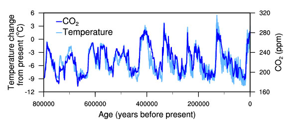
While the 1976 paper confirmed that orbital frequencies are present in the climate record, it also highlighted a paradox that remains one of the central unsolved problems in paleoclimatology. The ~100,000-year eccentricity cycle dominates the glacial record of the late Pleistocene — the past roughly 800,000 years — even though eccentricity is by far the weakest of the three orbital forcings in terms of insolation change. The variation in total annual solar energy caused by eccentricity changes is only about 0.2 percent, far too small to directly drive the massive glacial-interglacial temperature swings of 4–6°C in global mean temperature and 8–12°C in Antarctica.6, 9, 10
Numerous mechanisms have been proposed to explain the 100,000-year dominance. One class of models invokes nonlinear amplification through ice-sheet dynamics: once an ice sheet grows to a critical size, its own weight and internal dynamics make it susceptible to rapid collapse through processes such as marine ice-sheet instability, calving, and subglacial deformation. Under this view, the 100,000-year cycle reflects not the period of eccentricity forcing itself but rather the time required for an ice sheet to grow to its critical collapse threshold under the combined influence of obliquity and precession forcing, modulated by the eccentricity envelope.5, 6
A second class of models emphasises CO2 feedback. Ice core records from Antarctica show that atmospheric CO2 fell to approximately 180 parts per million during glacial maxima and rose to approximately 280 ppm during interglacials, tracking temperature changes with remarkable fidelity.9, 10 Ganopolski and Calov demonstrated with coupled ice-sheet–climate models that orbital forcing alone is insufficient to produce the full amplitude of Pleistocene deglaciations; the CO2 feedback is essential for tipping ice sheets into irreversible retreat once orbital conditions become favourable.12 The carbon cycle itself responds to orbital forcing through changes in ocean circulation, biological productivity, and the solubility of CO2 in seawater, creating a cascade of feedbacks that amplifies the weak eccentricity signal into the dominant periodicity of the ice-age record.
A third hypothesis, proposed by Huybers and Wunsch, challenges whether the ~100,000-year cycle is truly periodic at all. They argued that the late Pleistocene glacial terminations are more simply explained as occurring every second or third obliquity cycle (i.e., every ~80,000 or ~120,000 years), with the mean spacing of ~100,000 years being a statistical artefact of phase-locking to the obliquity beat rather than a response to eccentricity per se.19 Under this interpretation, obliquity — not eccentricity — remains the fundamental pacemaker even in the late Pleistocene, but the climate system's response is nonlinear, requiring multiple obliquity cycles to accumulate enough ice for a termination to occur.
The mid-Pleistocene transition
The 100,000-year problem is compounded by the observation that the late Pleistocene ~100 ka cyclicity is itself geologically recent. Before approximately 900,000–700,000 years ago, glacial cycles followed the 41,000-year obliquity rhythm, with ice sheets advancing and retreating modestly in tempo with the tilt cycle. The shift from 41 ka to ~100 ka dominant periodicity, accompanied by a dramatic increase in the amplitude of glacial-interglacial swings and a pronounced asymmetry (slow ice growth, rapid termination), is known as the mid-Pleistocene transition (MPT).8, 16
The MPT occurred without any corresponding change in orbital forcing — the eccentricity, obliquity, and precession parameters continued to vary on the same timescales before and after the transition. This rules out a purely external (astronomical) explanation and points to an internal change in the climate system's response to orbital forcing. Clark and colleagues proposed in 2006 that the key factor was the progressive removal of a thick regolith (weathered rock layer) from the Canadian and Scandinavian shields by repeated glacial erosion during the early Pleistocene. Once the regolith was stripped away, ice sheets formed on hard crystalline bedrock, which provided a stronger basal grip and allowed ice to grow thicker and more stable — thick enough to persist through obliquity-driven warm intervals that would previously have caused deglaciation. Only after two or three obliquity cycles of cumulative growth would the ice sheet become large enough for internal instabilities and CO2 feedbacks to trigger a catastrophic termination.8
An alternative explanation links the MPT to a long-term decline in atmospheric CO2 concentrations during the Plio-Pleistocene. As CO2 gradually fell below a critical threshold, the radiative forcing of the greenhouse effect diminished to the point where interglacial warmth was no longer sufficient to fully deglaciate the Northern Hemisphere during every obliquity peak. Lower CO2 effectively raised the bar for deglaciation, allowing ice sheets to survive longer and grow larger before the next termination.17, 18 Both hypotheses — regolith removal and CO2 decline — may contribute to the MPT, and distinguishing between them remains an active area of research.
Amplification and feedback mechanisms
Orbital forcing does not act on climate in isolation. The modest changes in insolation driven by the three Milankovitch parameters are amplified by a suite of positive feedback mechanisms that together produce the full glacial-interglacial climate swings recorded in the geological archive. Understanding these feedbacks is essential to explaining why relatively small orbital perturbations can drive global temperature changes of several degrees and ice volume changes equivalent to 120 metres of sea level.11, 12
The ice-albedo feedback is the most direct amplifier. Ice and snow reflect up to 80–90 percent of incoming solar radiation, compared to roughly 10 percent for dark ocean water or forested land. As ice sheets grow in response to reduced summer insolation, they increase Earth's overall albedo, reducing the amount of solar energy absorbed and promoting further cooling and ice growth. During deglaciation, the reverse applies: melting ice exposes dark surfaces, which absorb more energy and accelerate warming.4, 12
The carbon cycle feedback operates on longer timescales but is equally important. As the ocean cools during a glacial inception, its capacity to dissolve CO2 increases, drawing the gas out of the atmosphere. Changes in ocean circulation, the biological pump, and iron fertilisation of Southern Ocean productivity further lower atmospheric CO2 during glacials. The reduced greenhouse effect amplifies the initial orbital cooling. During terminations, warming oceans release CO2 back into the atmosphere, and the enhanced greenhouse effect helps drive deglaciation globally — critically, spreading the warming to the Southern Hemisphere even though the initial orbital forcing was strongest in the north.11
Additional feedbacks include changes in water vapour (itself the most powerful greenhouse gas, which amplifies any warming or cooling), changes in vegetation cover and dust loading, and the isostatic response of the lithosphere to ice loading and unloading, which affects ice-sheet stability. Ganopolski, Winkelmann, and Schellnhuber demonstrated in 2016 that the interplay between orbital insolation and CO2 concentration determines a critical threshold for glacial inception: below a certain CO2 level, even modest insolation minima can trigger ice-sheet growth, while above that level, inception fails regardless of orbital configuration. Their analysis suggested that anthropogenic CO2 emissions may have already delayed the next glacial inception by tens of thousands of years.13
Orbital forcing beyond the Quaternary
Although Milankovitch's theory was developed to explain Quaternary glaciations, orbital forcing has shaped Earth's climate far beyond the ice ages.
The recognition that the same astronomical cycles are recorded in pre-Quaternary sedimentary sequences has given rise to the discipline of cyclostratigraphy — the identification and dating of orbital cycles in the stratigraphic record — and its application to geological time calibration, known as astrochronology.21
In the Mesozoic and early Cenozoic, when Earth had no permanent polar ice sheets, orbital forcing still left a clear imprint on climate through its effects on the hydrological cycle, monsoon intensity, ocean productivity, and the distribution of organic-rich versus carbonate-rich sediments. The 405,000-year long eccentricity cycle has proven particularly valuable as a metronome for the geological time scale because its period is the most stable of all the Milankovitch cycles over geological time, remaining essentially constant for at least the past 250 million years.7, 21 Husson and colleagues used the 405 ka eccentricity cycle to astronomically calibrate the Maastrichtian stage of the Late Cretaceous, refining the age of the Cretaceous-Paleogene boundary with a precision unattainable by radiometric dating alone.14
In the Paleozoic, Horton and colleagues identified orbital periodicities in late Carboniferous and Permian climate proxy records, demonstrating that Milankovitch forcing operated during the late Paleozoic ice age in a manner analogous to the Quaternary, with obliquity and precession cycles pacing the advance and retreat of Gondwanan ice sheets.15 The orbital signal becomes progressively harder to detect in older rocks because of diagenetic alteration, the increasing uncertainty of radiometric age models, and the chaotic behaviour of the inner solar system, which means that the precise orbital solution cannot be calculated reliably beyond about 50–60 million years ago. Laskar and colleagues computed the most comprehensive long-term orbital solution (known as La2004) and demonstrated that while the long eccentricity cycle remains stable, the shorter eccentricity and precession cycles become unpredictable beyond the Eocene due to chaotic diffusion of the planetary orbits.7
Despite these limitations, geological evidence from tidal rhythmites and cyclic sedimentary sequences has been used to constrain the history of the Earth-Moon system and the Precambrian rotation rate. Williams analysed rhythmites from the ~620 Ma Elatina Formation in South Australia and inferred an obliquity cycle of approximately 30,000 years, consistent with a shorter Earth-Moon distance and faster lunar recession rate in the Neoproterozoic.20 Such studies illustrate that the Milankovitch framework extends in principle across the entirety of Earth history, even as the specific orbital parameters evolve over billions of years.
Modern significance
The astronomical theory of ice ages has significance that extends well beyond the reconstruction of past climates. By establishing the relationship between orbital forcing, ice-sheet response, and carbon cycle feedbacks, the Milankovitch framework provides a natural laboratory for understanding the sensitivity of the climate system to external perturbations — the same physics that governs glacial-interglacial cycles governs the response to anthropogenic greenhouse gas emissions.11, 13
The ice core record demonstrates that for the past 800,000 years, atmospheric CO2 never exceeded approximately 300 parts per million during interglacials.9 The current concentration, exceeding 420 ppm, is without precedent in at least that interval and probably in several million years. Ganopolski and colleagues' modelling work suggests that even at pre-industrial CO2 levels the next glacial inception would not occur for approximately 50,000 years due to an unusually weak future insolation minimum, and that the anthropogenic addition of CO2 may suppress glacial inception for at least 100,000 years beyond that.13 The Milankovitch cycles have not ceased — the orbital parameters continue their clockwork variation — but the climate system's response to them has been fundamentally altered by a forcing that operates orders of magnitude faster than any natural orbital perturbation.13
Astrochronology, meanwhile, continues to refine the geological time scale with a precision that no other dating method can achieve. By tuning sedimentary records to the computed orbital solution, geologists can assign absolute ages to stratigraphic boundaries with uncertainties of a few thousand years — even in rocks tens of millions of years old. This capacity has transformed stratigraphy from a relative science into a quantitative one and has enabled high-resolution studies of evolutionary rates, extinction timing, and ocean-atmosphere dynamics across deep time.21, 22
References
On the structure and origin of major glaciation cycles. 1. Linear responses to Milankovitch forcing
The Mid-Pleistocene Transition: characteristics, mechanisms, and implications for long-term changes in atmospheric pCO2
Integrated summer insolation forcing and 40,000-year glacial cycles: the perspective from an ice-free world