Overview
- Biostratigraphy uses the distribution of fossils in sedimentary rock to date, subdivide, and correlate strata across vast distances, building on William Smith's early nineteenth-century discovery that each rock layer contains a distinctive and predictable succession of fossil species.
- Good index fossils — organisms with wide geographic range, short temporal range, high abundance, and easy identification — provide the primary markers for defining biozones, and groups such as trilobites, graptolites, ammonites, conodonts, and foraminifera have each served as the backbone of stratigraphic correlation through successive geologic eras.
- Modern quantitative methods including constrained optimization (CONOP), unitary associations, and graphic correlation now allow biostratigraphers to integrate thousands of fossil occurrences computationally, achieving sub-million-year resolution and underpinning the calibration of the international geologic time scale.
Biostratigraphy is the branch of stratigraphy that uses the distribution of fossils in sedimentary rock to date, subdivide, and correlate strata. It rests on a single foundational observation: fossil species appear and disappear in a consistent, non-repeating order throughout the geologic record, so that each interval of rock contains a distinctive assemblage of organisms that can be used to identify its relative age and match it to equivalent strata elsewhere.5, 22 Since its formalization in the early nineteenth century, biostratigraphy has served as the primary means of correlating marine and terrestrial sedimentary sequences across continents and ocean basins, and it remains indispensable even in an era of radiometric dating and geochemical chemostratigraphy. The international geologic time scale — with its familiar hierarchy of eras, periods, epochs, and stages — was built overwhelmingly on biostratigraphic foundations, and the majority of the boundaries that define its subdivisions are anchored to the first or last appearances of particular fossil species.6, 18
The fossils most useful for this purpose are called index fossils (or guide fossils): species that were geographically widespread, temporally short-lived, numerically abundant, and morphologically distinctive. Different groups of organisms have dominated biostratigraphic practice in different intervals of geologic time — trilobites in the Cambrian, graptolites in the Ordovician and Silurian, ammonites in the Jurassic and Cretaceous, planktonic foraminifera and calcareous nannofossils in the Cenozoic — each group contributing the particular combination of rapid evolution, wide dispersal, and preservational robustness that makes high-resolution correlation possible.6, 7, 12
Historical foundations
The intellectual origins of biostratigraphy lie in the work of the English surveyor and canal engineer William Smith (1769–1839). While supervising the excavation of the Somerset Coal Canal in the 1790s, Smith noticed that the sedimentary rock layers exposed in the canal cuts and surrounding quarries always occurred in the same vertical order and that each layer contained a characteristic set of fossils that was different from the layers above and below it. By the late 1790s he had recognized what would later be called the principle of faunal succession: that strata could be identified and correlated across large distances not merely by their lithology — which might change laterally — but by the fossils they contained.1, 2

In 1815, Smith published his landmark geological map of England and Wales, the first large-scale geological map to use fossil content as a basis for distinguishing and correlating rock units across an entire country. The accompanying explanatory text and his subsequent work Strata Identified by Organized Fossils (1816–1819) illustrated the diagnostic fossils of each formation, providing a practical field guide for applying his principle.1, 2 Smith's insight that fossils, rather than rock type, were the most reliable key to stratigraphic correlation was revolutionary. Two limestone beds hundreds of kilometres apart might look identical in hand specimen, but if one contained the ammonite Dactylioceras and the other contained Hildoceras, they belonged to different intervals of time.
The formalization of biostratigraphy into a rigorous system of zones came several decades later through the work of the German palaeontologist Albert Oppel (1831–1865). In his monograph Die Juraformation Englands, Frankreichs und des südwestlichen Deutschlands (1856–1858), Oppel divided the Jurassic into a sequence of zones defined not by single species but by associations of species whose overlapping ranges identified narrow time intervals.3, 4 He recognized 33 zones across the Jurassic, most named after characteristic ammonite species, and demonstrated that the same zonal sequence could be traced from England through France to southwestern Germany. Oppel's zonal concept introduced the idea that a biostratigraphic unit should be defined by the co-occurrence of multiple taxa, an approach that increased both the precision and the reproducibility of fossil-based correlation.3, 19
What makes a good index fossil
Not all fossils are equally useful for dating and correlating rock layers. A good index fossil (also called a guide fossil or zone fossil) must satisfy several criteria simultaneously. First, it must have had a wide geographic distribution during its lifetime, so that it can be found in sedimentary sequences across multiple continents or ocean basins. Organisms that lived in the open ocean, such as planktonic foraminifera, graptolites, and ammonites, are particularly well suited because ocean currents dispersed them broadly.5, 22
Second, the species must have had a short temporal range — it must have evolved, proliferated, and gone extinct within a geologically brief interval. The shorter the species' duration, the narrower the time window it can diagnose. Rapidly evolving lineages that underwent frequent speciation events, such as ammonites and planktonic foraminifera, produce species whose ranges span only one to three million years or less, enabling fine-scale subdivision of geologic time.11, 12
Third, the fossil must occur in high abundance, so that the probability of finding specimens in any given outcrop or drill core is high. Microfossils such as foraminifera and calcareous nannofossils are recovered in enormous numbers from even small rock or sediment samples, making them extraordinarily practical for petroleum exploration, ocean drilling, and other subsurface applications where sample volumes are limited.14, 22
Fourth, the fossil must be easily identifiable, with distinctive morphological features that allow reliable identification even by non-specialists. Ammonites, with their coiled shells bearing ornate ribbing and suture patterns, and trilobites, with their segmented exoskeletons showing diagnostic features of the cephalon and pygidium, both meet this requirement well.6, 7 Finally, the fossil should ideally be independent of facies — found in multiple rock types and depositional environments — so that its occurrence is controlled by time rather than by local ecological conditions.5
Types of biozones
The fundamental unit of biostratigraphy is the biozone (or zone): a body of rock defined and characterized by its fossil content. The International Stratigraphic Guide, maintained by the International Subcommission on Stratigraphic Classification, recognizes five principal types of biozones, each defined by different criteria.5
A taxon-range zone (or range zone) encompasses the total stratigraphic interval over which a particular species or taxon is known to occur. Its lower boundary is defined by the taxon's lowest (first) occurrence and its upper boundary by the taxon's highest (last) occurrence. A concurrent-range zone is a variant in which the zone is defined by the overlap in the ranges of two taxa, and the boundaries are set by the first occurrence of the younger taxon and the last occurrence of the older one. Concurrent-range zones are narrower than individual taxon-range zones and therefore provide higher stratigraphic resolution.5, 22
An interval zone is the body of strata between two specified biohorizons — typically the first or last appearance of particular taxa — without requiring that any specific taxon be present throughout the interval. This type of zone is especially useful when the defining taxon is rare or patchily distributed, because the zone boundaries are drawn at well-defined bioevents rather than at ranges of continuous occurrence.5
An assemblage zone is defined by a distinctive association of three or more taxa that, taken together, distinguish the strata from adjacent zones. No single species need span the entire zone; rather, the combination of species present is diagnostic. Assemblage zones are particularly useful in terrestrial sequences where individual species may have limited geographic ranges but characteristic faunal or floral communities recur predictably.5, 22
An abundance zone (or acme zone) is defined by the interval in which a particular taxon reaches its maximum relative or absolute abundance, even though the taxon may range above and below the zone. Abundance zones are used when a species' peak proliferation is a more reliable and reproducible signal than its first or last occurrence, which may be affected by sampling gaps or ecological exclusion. The diatom Ethmodiscus rex and certain planktonic foraminiferal species have been used to define abundance zones in deep-sea sediments.5, 15
A fifth type, the lineage zone (or phylozone), is based on successive species within an evolutionary lineage, with boundaries drawn at the evolutionary appearance of each successive descendant species. Lineage zones are especially powerful because they reflect genuine evolutionary change rather than local ecological factors, but they require well-documented ancestor-descendant relationships, which are available for only a fraction of fossil groups.5
Key index fossils through geologic time
Different fossil groups have served as the primary biostratigraphic tools in different intervals of the Phanerozoic, reflecting the evolutionary diversification, ecological dominance, and preservational characteristics of each group during its period of greatest utility.
Trilobites are the preeminent index fossils of the Cambrian Period and remain important throughout the lower Palaeozoic. These marine arthropods appeared in the early Cambrian around 521 million years ago, underwent rapid diversification, and persisted until their extinction at the end of the Permian, approximately 252 million years ago. Their utility as index fossils stems from their morphological diversity, their abundance in shallow marine sediments, and the fact that their calcified exoskeletons were moulted repeatedly during growth, producing multiple preservable elements per individual. Most of the Cambrian is subdivided using trilobite-based biozones, and 13 of the Cambrian stage boundaries in the current geologic time scale are defined or correlated primarily using trilobite first appearances.6, 7
Graptolites — colonial hemichordates that lived as planktonic or epiplanktonic organisms in the Palaeozoic oceans — are the primary biostratigraphic tool for the Ordovician, Silurian, and Lower Devonian, particularly in deep-water and offshore marine facies where trilobites and other benthic organisms are rare or absent. Graptolites evolved rapidly, producing a succession of short-lived species, and their planktonic habit ensured worldwide distribution. The Ordovician and Silurian together are divided into approximately 60 to 70 graptolite biozones, many with durations of less than one million years, providing one of the highest-resolution biostratigraphic frameworks in the entire Phanerozoic. Thirteen Global Stratotype Section and Point (GSSP) boundaries are defined by first appearance datums of graptolite species.8
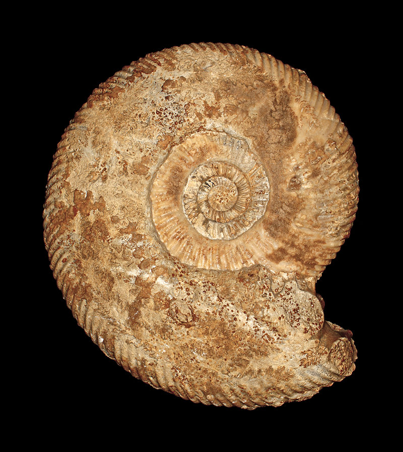
Ammonites — extinct cephalopod molluscs with external, chambered shells — are the dominant index fossils of the Mesozoic Era, particularly the Jurassic and Cretaceous periods. Following a near-total extinction at the end of the Triassic, ammonites underwent an explosive radiation in the Early Jurassic that produced hundreds of rapidly evolving, morphologically distinctive lineages. The Jurassic alone is subdivided into approximately 60 to 70 ammonite zones, many with durations of 0.5 to 1.5 million years, making ammonite biostratigraphy one of the most refined of all fossil-based correlation schemes.3, 11 The Cretaceous is similarly well zoned, with ammonite-based biozones providing the primary framework for marine correlation across Europe, the Americas, and beyond.10
Planktonic foraminifera and calcareous nannofossils are the principal index fossils of the Cenozoic Era. Planktonic foraminifera — single-celled protists with calcium carbonate shells — evolved rapidly during the Late Cretaceous and Cenozoic, producing a succession of short-lived species that are recovered in vast numbers from deep-sea sediment cores and outcrop samples. The standard tropical planktonic foraminiferal zonation recognizes over 70 biozones for the Cenozoic, with many zones spanning less than two million years.12 Calcareous nannofossils, the tiny calcareous plates (coccoliths) shed by coccolithophore algae, provide an independent and complementary zonation: the Martini (1971) standard nannofossil zonation divides the Cenozoic into 46 zones (25 for the Palaeogene, 21 for the Neogene), and subsequent revisions have further refined this framework.13
Major index fossil groups and their biostratigraphic application6, 7, 8, 12
| Fossil group | Primary interval | Approximate number of biozones | Typical zone duration | Key advantage |
|---|---|---|---|---|
| Trilobites | Cambrian–Ordovician | ~50–60 (Cambrian) | 1–5 Myr | Morphological diversity; abundant in shelf facies |
| Graptolites | Ordovician–Lower Devonian | ~60–70 | <1 Myr | Planktonic; global distribution; rapid evolution |
| Conodonts | Late Cambrian–Triassic | ~80–100+ | 0.5–3 Myr | Acid-resistant; recoverable from diverse lithologies |
| Ammonites | Jurassic–Cretaceous | ~120–140 (Jurassic + Cretaceous) | 0.5–1.5 Myr | Rapid speciation; ornate, easily distinguished shells |
| Planktonic foraminifera | Late Cretaceous–Recent | ~70+ (Cenozoic) | 1–3 Myr | Pelagic; enormous abundance; recoverable from cores |
| Calcareous nannofossils | Jurassic–Recent | ~46 (Cenozoic, Martini 1971) | 1–3 Myr | Microscopic; vast numbers per gram of sediment |
Conodont biostratigraphy
Conodonts occupy a unique position in biostratigraphy. These small, tooth-like phosphatic elements were produced by an extinct group of eel-like marine vertebrates (or near-vertebrates) that ranged from the late Cambrian to the end of the Triassic, a span of approximately 300 million years.9 Because conodont elements are composed of calcium phosphate (apatite) rather than calcium carbonate, they resist dissolution in acidic environments and can be extracted from limestone and dolostone samples by dissolving the carbite matrix in weak acids — a processing technique that yields hundreds to thousands of identifiable elements from a single kilogram of rock. This acid-resistant property makes conodonts recoverable from a far wider range of lithologies than most other fossil groups.9, 6
Conodont biostratigraphy provides the primary framework for subdividing the upper Cambrian through the Triassic. The animals evolved rapidly, producing morphologically distinctive element types that changed through time in well-documented lineages, and their pelagic or nektonic lifestyle ensured broad geographic distribution. As a result, more GSSP boundaries in the Palaeozoic and Triassic are defined using conodont first appearance datums than by any other single fossil group. The base of the Ordovician System, for example, is defined by the first appearance of the conodont Iapetognathus fluctivagus, and the base of the Triassic is defined by the first appearance of Hindeodus parvus.6, 9
The integration of conodont data with graptolite, chitinozoan, and trilobite biostratigraphy has been a major focus of Palaeozoic stratigraphic research. Because conodonts occur in shallow-water carbonate facies where graptolites are typically absent, and graptolites occur in deep-water shale facies where conodonts may be rare, the two groups provide complementary coverage of the environmental spectrum. Where both groups co-occur, their combined data substantially improve the resolution and reliability of stratigraphic correlation.8, 9
Microfossils and petroleum geology
The petroleum industry has been one of the principal drivers of advances in biostratigraphy, particularly in the study of microfossils. When drilling an exploration well into deep subsurface formations, biostratigraphy is often the most practical — and sometimes the only — method of determining the age and stratigraphic position of the rocks being penetrated. Drill cuttings brought to the surface during drilling are routinely examined for microfossils, which provide real-time age control that guides decisions about well depth, casing points, and formation correlation.14, 21
Three microfossil groups dominate petroleum biostratigraphy: foraminifera, calcareous nannofossils, and palynomorphs (pollen, spores, and dinoflagellate cysts). Planktonic foraminifera and nannofossils are used for long-distance age correlation in marine sequences, while benthic foraminifera provide additional information about palaeobathymetry and palaeoenvironment — critical parameters for reconstructing the depositional history of sedimentary basins and predicting the distribution of reservoir, seal, and source rocks.14, 21 Palynomorphs are especially valuable in non-marine and marginal marine sediments where calcareous microfossils may be absent.
The practical utility of microfossil biostratigraphy in petroleum exploration extends beyond simple age determination. By identifying the biostratigraphic zones penetrated by a well and comparing them with zones in nearby wells, geologists can detect unconformities (gaps in the record representing periods of erosion or non-deposition), identify faults that have repeated or omitted stratigraphic sections, and correlate reservoir horizons across a field or basin. The development of high-resolution biostratigraphic schemes for prolific petroleum provinces such as the Gulf of Mexico, the North Sea, and the Niger Delta has been a major area of applied micropalaeontological research for over a century.14, 21
Biostratigraphy and chronostratigraphy
Biostratigraphy and chronostratigraphy are closely related but conceptually distinct disciplines. Biostratigraphy classifies rock based on its fossil content; chronostratigraphy classifies rock based on the time during which it was deposited. The geologic time scale is fundamentally a chronostratigraphic construct — its stages, series, and systems are defined as bodies of rock deposited during specific intervals of time — but the boundaries between those chronostratigraphic units are, in the great majority of cases, defined using biostratigraphic criteria.18, 20
The modern mechanism for defining chronostratigraphic boundaries is the Global Boundary Stratotype Section and Point (GSSP), an internationally agreed-upon reference point in a specific stratigraphic section that fixes the lower boundary of a stage. The GSSP is colloquially known as a "golden spike." The primary criterion for selecting a GSSP is typically the first appearance datum (FAD) of a fossil species — a biostratigraphic event — supplemented where possible by additional markers such as magnetic polarity reversals, stable isotope excursions, or radiometric dates that aid correlation.18, 23 Of the approximately 70 GSSPs currently ratified by the International Commission on Stratigraphy, the large majority use a biostratigraphic marker as their primary defining criterion.6, 18
There is, however, an important conceptual distinction between biostratigraphic and chronostratigraphic boundaries. A biostratigraphic boundary — such as the first appearance of a species — is inherently diachronous in principle: a species that evolves in one region may take thousands or millions of years to disperse to other parts of the world, so its first local appearance in different sections may represent slightly different moments in time. Chronostratigraphic boundaries, by contrast, are defined to be synchronous — representing a single instant of time worldwide. The GSSP system resolves this tension by fixing the boundary at a single point in a single section, which is then correlated to other sections using the best available combination of biostratigraphic, magnetostratigraphic, and chemostratigraphic evidence.18, 19
Modern quantitative biostratigraphy

Traditional biostratigraphy relied on the expert judgment of individual palaeontologists to establish the order of fossil appearances and disappearances, define zones, and correlate sections. Beginning in the 1960s, researchers developed quantitative methods that use mathematical algorithms and computational power to integrate large volumes of biostratigraphic data from multiple sections and produce optimized composite sequences with higher resolution and greater objectivity than manual methods could achieve.15, 17
Graphic correlation, introduced by Alan Shaw in 1964, was the first widely adopted quantitative approach. Shaw's method involves plotting the stratigraphic positions of first and last occurrences of fossil taxa in two sections on an x-y graph, then fitting a line of correlation through the points. The slope and position of this line express the relative rates of sedimentation between the two sections, and departures from the line identify range truncations, hiatuses, or misidentifications. A composite reference section is built iteratively by correlating additional sections to the composite and extending the known ranges of taxa. Graphic correlation remains widely used in petroleum exploration because of its visual clarity and its ability to incorporate diverse data types — radiometric dates, magnetic reversals, and geochemical events — alongside fossil occurrences.15, 17
Constrained optimization (CONOP), developed by Peter Sadler and colleagues, is a multidimensional extension of graphic correlation that uses simulated annealing algorithms to find the optimal ordering and spacing of biostratigraphic events across an unlimited number of sections simultaneously. CONOP treats the construction of a composite sequence as an optimization problem: it seeks the event ordering that requires the minimum total adjustment to the observed local ranges across all input sections, subject to the constraint that any viable solution must reproduce all observed taxon co-occurrences. The method has been used to build high-resolution composite range charts for Ordovician graptolites, Cambrian trilobites, Cenozoic planktonic foraminifera, and many other groups, and it has been directly incorporated into the construction of the Geologic Time Scale 2012 and 2020.6, 15, 20
The unitary associations method, developed by Jean Guex and Eric Davaud, takes a different approach rooted in graph theory. Rather than seeking an optimal ordering of individual events, unitary associations identifies maximal sets of taxa that are mutually compatible — that is, whose observed stratigraphic ranges overlap in at least one section — and uses these sets as the building blocks of a composite biochronological scale. The method is particularly effective at resolving conflicting range data and producing discrete, reproducible biozones from complex datasets with large numbers of taxa and sections.16, 24
These quantitative methods have transformed biostratigraphy from a largely qualitative, expert-dependent practice into a data-intensive discipline capable of processing thousands of fossil occurrences from hundreds of sections. By integrating biostratigraphic data with radiometric dates, magnetostratigraphy, and astrochronology (the calibration of sedimentary cycles to astronomical forcing), modern biostratigraphers achieve temporal resolutions of a few hundred thousand years or better in many parts of the Phanerozoic — resolutions that would have been unimaginable to William Smith, yet rest firmly on the same principle of faunal succession he recognized more than two centuries ago.6, 15, 20
References
Memoir to the Map and Delineation of the Strata of England and Wales, with Part of Scotland
Cambrian trilobite biostratigraphy and its role in developing an integrated history of the Earth system
Graptolites in biostratigraphy: the primary tool for subdivision and correlation of Ordovician, Silurian, and Lower Devonian offshore marine successions
From Oppel to Callomon (and beyond): building a high-resolution ammonite-based biochronology for the Jurassic System
Review and revision of Cenozoic tropical planktonic foraminiferal biostratigraphy and calibration to the geomagnetic polarity and astronomical time scale
History, philosophy, and application of the Global Stratotype Section and Point (GSSP)