Overview
- Earth's magnetic field has reversed polarity hundreds of times over geological history, and each reversal is permanently recorded in volcanic rocks and ocean-floor basalts, creating a global barcode of normal and reversed magnetization that extends back more than 170 million years.
- The geomagnetic polarity timescale, calibrated against radiometric dates from lava flows and seafloor magnetic anomalies, provides an independent chronological framework that confirms deep time and enables precise correlation of sedimentary sequences across every continent and ocean basin.
- Marine magnetic anomalies — the symmetric stripes of alternating magnetization on either side of mid-ocean ridges — independently verify both the polarity timescale and the theory of seafloor spreading, linking geomagnetism, plate tectonics, and deep-time chronology into a single, mutually reinforcing framework.
Earth's magnetic field has not always pointed in the same direction. Over geological time, the field has repeatedly reversed its polarity, with the magnetic north and south poles exchanging positions in episodes that are permanently recorded in the magnetization of rocks worldwide. The study of these reversals has produced one of the most powerful chronological tools in the earth sciences: the geomagnetic polarity timescale (GPTS), a calibrated sequence of normal and reversed polarity intervals extending back more than 170 million years.8, 10 Because each reversal is a geologically instantaneous, globally synchronous event, the pattern of reversals functions as a temporal barcode that can be read in lava flows, sedimentary sequences, and ocean-floor basalts on every continent and in every ocean basin. The GPTS provides independent confirmation of deep time that is entirely separate from — and mutually consistent with — radiometric dating, stratigraphy, and the fossil record.12, 22
Discovery of magnetic reversals
The idea that Earth's magnetic field could reverse its polarity was first suggested by the French physicist Bernard Brunhes in 1906. While studying Pliocene lava flows in the Massif Central of south-central France, Brunhes discovered that certain basalts were magnetized in a direction approximately antiparallel to the present-day geomagnetic field — that is, their magnetic north pointed toward the geographic south pole. He concluded that these rocks had cooled and solidified at a time when Earth's magnetic field was oriented opposite to its present configuration.1 This was a radical proposal, and it was met with widespread skepticism. Many geologists suspected that the anomalous magnetization resulted from unusual mineralogy or chemical alteration rather than a genuine reversal of the planetary field.
The Japanese geophysicist Motonori Matuyama provided the next critical advance in 1929. Working with basalt samples from Japan, Korea, and Manchuria, Matuyama demonstrated that rocks of Pleistocene age were magnetized in the same direction as the present field, while older basalts of late Pliocene and early Pleistocene age were consistently magnetized in the reverse direction. Crucially, Matuyama recognized that the transition between normal and reversed magnetization correlated with geological age rather than geographic location or rock composition, strongly implying that the field itself had reversed rather than that individual rocks had acquired aberrant magnetizations.2 This correlation between polarity and age was the first empirical evidence that reversals were real, global phenomena tied to a specific moment in geological time.
Definitive proof came in the early 1960s, when Allan Cox, Richard Doell, and Brent Dalrymple at the United States Geological Survey combined potassium-argon (K-Ar) radiometric dating with paleomagnetic measurements of young lava flows from around the world. By dating the same lava flows whose magnetic polarity they had measured, they showed that all normally magnetized lavas fell within certain age ranges and all reversely magnetized lavas fell within others, regardless of where on Earth they were sampled.3 By 1964, they had constructed the first radiometrically calibrated polarity timescale for the past 3.6 million years, identifying four major polarity intervals that they named after pioneers of geomagnetism: the Brunhes Normal Chron, the Matuyama Reversed Chron, the Gauss Normal Chron, and the Gilbert Reversed Chron.3, 4
How reversals are recorded in rocks
The physical mechanism by which rocks preserve a record of the geomagnetic field was first explained theoretically by the French physicist Louis Néel, whose work on the magnetic properties of fine-grained minerals earned him the Nobel Prize in Physics in 1970. Néel showed that when a lava flow cools through a critical temperature known as the Curie point (approximately 580 °C for magnetite, the most common magnetic mineral in basalt), the magnetic domains within ferromagnetic mineral grains become locked in alignment with the ambient magnetic field. This acquired magnetization, called thermoremanent magnetization (TRM), is extremely stable and can persist for billions of years provided the rock is not subsequently reheated above the Curie point.14 TRM is the primary recording mechanism in volcanic rocks, and it faithfully preserves both the direction and the relative intensity of the geomagnetic field at the time the lava solidified.22, 23
Sedimentary rocks acquire their magnetization through a different process. As fine-grained sediment settles through a water column — in a lake, an ocean, or a floodplain — detrital grains of magnetite and other ferromagnetic minerals rotate to align with the ambient field before being locked in place by compaction and cementation. This detrital remanent magnetization (DRM) is generally weaker than TRM and can be subject to post-depositional disturbance, but in fine-grained, slowly deposited sequences such as deep-sea oozes and lacustrine clays, DRM provides a continuous, high-resolution record of geomagnetic polarity changes that complements the discontinuous record from lava flows.12, 13 The great advantage of sedimentary records is their continuity: a single deep-sea core can span millions of years of uninterrupted deposition, capturing not only the polarity of the field but also the transitional behaviour of the field during a reversal.12
A third mechanism, chemical remanent magnetization (CRM), occurs when new magnetic minerals grow within a rock through chemical alteration or diagenesis at temperatures below the Curie point. CRM can either reinforce the original magnetization or, if the chemical alteration occurs long after deposition, overprint it with a younger magnetic signature. Paleomagnetic studies routinely employ stepwise thermal or alternating-field demagnetization to strip away secondary CRM components and isolate the primary magnetization acquired at the time of formation.22
The geomagnetic polarity timescale
The GPTS is a calibrated chronological framework that assigns numerical ages to each polarity reversal in Earth's magnetic history. The timescale is constructed by integrating three independent data sources: radiometric ages from dated lava flows, the pattern of marine magnetic anomalies recorded in ocean-floor basalts, and astronomical tuning of sedimentary sequences to orbital cycles.8, 9, 10

The modern GPTS has its foundation in the work of Cande and Kent, who in 1992 published a comprehensive polarity timescale (designated CK92) for the Late Cretaceous and Cenozoic — the past approximately 83 million years — by combining marine magnetic anomaly profiles from the world's ocean basins with a set of radiometrically dated calibration points.8 They refined this timescale in 1995 (CK95) using improved 40Ar/39Ar ages and astronomical calibrations, producing the framework that remains the basis of current versions.9 The most recent iteration, incorporated into the Geologic Time Scale 2020, extends the calibrated GPTS through the Jurassic and into the Middle Jurassic, approximately 170 million years ago, using magnetic anomaly data from the oldest surviving ocean floor in the western Pacific.10, 17, 21
The temporal resolution of the GPTS varies across geological time. For the past five million years, where numerous lava flows have been dated by K-Ar and 40Ar/39Ar methods, individual reversals are constrained to within a few thousand years.3, 4, 15 For the Cenozoic and Late Cretaceous, the combination of marine magnetic anomaly profiles and astronomical tuning provides a resolution of approximately 10,000 to 100,000 years.9 For the Jurassic, where the ocean-floor record is incomplete and radiometric tie points are fewer, uncertainties increase to several hundred thousand years.24 Despite these variations, the GPTS provides a globally consistent chronological framework that is independent of and complementary to biostratigraphy and radiometric dating.
Named chrons and superchrons
The fundamental unit of the GPTS is the chron, a continuous interval of predominantly one polarity. Chrons are numbered sequentially backward from the present, with the prefix "C" denoting the Cenozoic and Late Cretaceous portion of the timescale and "M" denoting the Mesozoic (Jurassic and Early Cretaceous) portion. The four youngest chrons, spanning the past approximately 5.3 million years, bear the names of pioneers in the study of geomagnetism and are universally used as reference intervals in Plio-Pleistocene stratigraphy.3, 4, 10
The Brunhes Normal Chron (C1n) encompasses the present period of normal polarity, beginning at approximately 780,000 years ago and extending to the present day.4, 15 The Matuyama Reversed Chron (C1r through C2n) spans from approximately 780,000 to 2.6 million years ago and is predominantly reversed, though it contains several short normal-polarity subchrons, including the Jaramillo (approximately 1.07 to 0.99 million years ago) and the Olduvai (approximately 1.95 to 1.78 million years ago), both of which are important marker horizons in early human evolution and stratigraphy.3, 4, 12 The Gauss Normal Chron extends from approximately 2.6 to 3.6 million years ago, and the Gilbert Reversed Chron extends from approximately 3.6 to 5.3 million years ago.3, 10
Major geomagnetic polarity chrons of the past 5.3 million years3, 4, 10
| Chron | Polarity | Age range (Ma) | Named after |
|---|---|---|---|
| Brunhes (C1n) | Normal | 0 – 0.78 | Bernard Brunhes |
| Matuyama (C1r–C2n) | Reversed | 0.78 – 2.60 | Motonori Matuyama |
| Gauss (C2An) | Normal | 2.60 – 3.60 | Carl Friedrich Gauss |
| Gilbert (C2Ar–C3n) | Reversed | 3.60 – 5.33 | William Gilbert |
Beyond these named chrons, the GPTS records hundreds of polarity intervals stretching back through the Mesozoic. One of the most striking features of the timescale is the Cretaceous Normal Superchron (also called the Cretaceous Quiet Zone), a prolonged interval of approximately 38 million years during which the geomagnetic field maintained normal polarity without a single reversal. The Cretaceous Normal Superchron spans from approximately 121 to 83 million years ago (chrons C34n to the end of the Cretaceous quiet interval), making it the longest known period without a reversal in the past 170 million years.11, 18 The cause of superchrons remains debated, but they are thought to reflect changes in the dynamics of the outer core, possibly linked to large-scale mantle convection patterns and the thermal insulation of the core by deep mantle structures.18, 20
Magnetostratigraphy as a correlation tool
Magnetostratigraphy is the application of the GPTS to the dating and correlation of sedimentary and volcanic sequences. The technique works because each reversal is recorded simultaneously in rocks forming anywhere on Earth, creating a globally synchronous set of marker horizons. By measuring the magnetic polarity of a sequence of rock layers and matching the observed pattern of normal and reversed intervals to the known GPTS, geologists can assign numerical ages to the sequence without requiring radiometric dating of every individual layer.12
The power of magnetostratigraphy was first demonstrated in the mid-1960s, when Neil Opdyke and colleagues measured the magnetic polarity of deep-sea sediment cores from the Southern Ocean and found that the pattern of normal and reversed zones in the cores matched the polarity timescale that Cox, Doell, and Dalrymple had constructed independently from dated lava flows on land.13 This agreement between two completely independent data sets — volcanic rocks dated by K-Ar on land and sediment cores from the deep ocean — was powerful confirmation that the reversals were real, global events and that the polarity timescale was a reliable chronological tool.12, 13
Today, magnetostratigraphy is used routinely to date and correlate sedimentary sequences on every continent. It is particularly valuable in settings where biostratigraphic markers are absent or poorly preserved, such as continental red beds, loess sequences, and lacustrine deposits. In the Chinese Loess Plateau, for example, magnetostratigraphic analysis has established a detailed chronology of wind-blown dust deposition spanning the past 2.6 million years, providing one of the longest and most complete terrestrial climate records on Earth.12, 22 In East African rift basins, magnetostratigraphy has been instrumental in dating the sedimentary layers that contain early hominin fossils, providing precise age constraints for critical sites such as Olduvai Gorge, where the Olduvai subchron was in fact named for the normal-polarity interval first identified in its sediments.12
The technique is most effective when the sedimentary sequence can be independently tied to the GPTS through at least one radiometric date or biostratigraphic datum. Without such a tie point, the polarity pattern in a given section can sometimes be matched to more than one segment of the GPTS. However, when combined with biostratigraphy, radiometric dating, or astronomical tuning, magnetostratigraphy provides a level of chronological precision that few other methods can match in pre-Quaternary sequences.10, 12
Marine magnetic anomalies and seafloor spreading
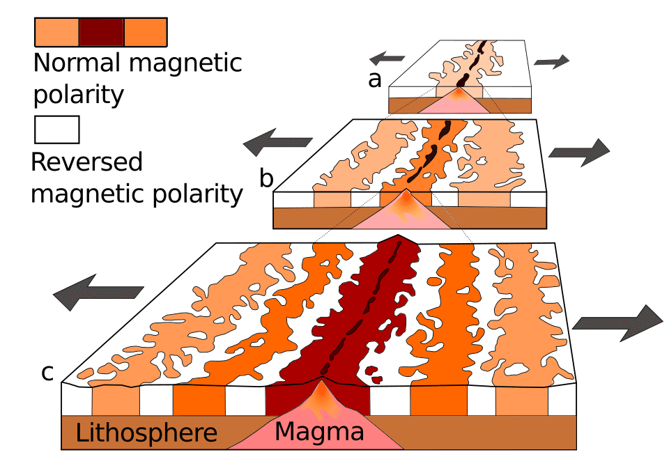
The most dramatic confirmation of the GPTS came not from rocks on land but from the floor of the ocean. In 1963, Frederick Vine and Drummond Matthews at the University of Cambridge proposed that the symmetric pattern of magnetic anomalies observed on either side of the Mid-Atlantic Ridge could be explained if new oceanic crust, formed at the ridge by seafloor spreading, acquired a thermoremanent magnetization aligned with the ambient geomagnetic field and was then carried away from the ridge axis by plate motion.5 When the field was normal, the newly formed basalt would be magnetized in the normal direction; when the field reversed, the new basalt would be magnetized in the reverse direction. The result would be a series of alternating stripes of normal and reversed magnetization, symmetrically disposed about the ridge axis, forming a magnetic barcode that recorded the history of geomagnetic reversals on the ocean floor. The same hypothesis was independently proposed by Lawrence Morley in Canada, though his manuscript was initially rejected by the journals Nature and the Journal of Geophysical Research before Vine and Matthews published their version.7
Vine tested the hypothesis decisively in 1966 by showing that the magnetic anomaly profiles from the Juan de Fuca Ridge off the coast of the Pacific Northwest could be matched in detail to the independently derived polarity timescale of Cox, Doell, and Dalrymple. The correspondence was exact: each anomaly stripe on the ocean floor matched a specific polarity chron, and the width of each stripe was proportional to the duration of that chron multiplied by the spreading rate of the ridge.6 This result simultaneously confirmed three major geological hypotheses: that the seafloor was spreading, that the geomagnetic field had reversed repeatedly, and that the polarity timescale derived from dated lava flows on land was correct.
Marine magnetic anomalies have since been mapped across every major ocean basin and have extended the GPTS far beyond the range accessible from land-based lava flows alone. The oldest identifiable marine magnetic anomalies are found in the western Pacific, where Jurassic-age ocean floor preserves anomalies dating back approximately 170 million years.17 Beyond that age, no ocean floor survives — the older crust has been consumed by subduction — and the Mesozoic portion of the GPTS must be reconstructed from magnetized sedimentary sequences on land.24 The marine magnetic anomaly record is one of the most compelling demonstrations of deep time in all of geology, for it requires that the ocean floor has been continuously created and destroyed over hundreds of millions of years, with each cycle faithfully recording the reversals of Earth's magnetic field.6, 8
The Brunhes-Matuyama reversal
The most recent full reversal of Earth's magnetic field, the Brunhes-Matuyama boundary, occurred approximately 780,000 years ago and serves as one of the most widely used chronostratigraphic markers in Quaternary geology.4, 15 The reversal has been identified and dated in lava flows on every continent, in deep-sea sediment cores from every ocean basin, in loess sequences in China and Central Europe, and in lacustrine deposits from East Africa to the western United States. Its global ubiquity and chronological precision make it an anchor point for correlating geological, paleoclimate, and archaeological records across the late Quaternary.12, 16
The age of the Brunhes-Matuyama reversal has been determined by multiple independent methods. 40Ar/39Ar dating of transitionally magnetized lava flows in Maui (Hawaii), Tahiti, and Chile has yielded ages clustering around 780,000 years.15 Astronomical tuning of deep-sea oxygen-isotope records — in which the sedimentary record of glacial and interglacial cycles is matched to the calculated variations in Earth's orbital parameters — places the reversal at approximately 780,000 to 781,000 years ago, in excellent agreement with the radiometric dates.16 This concordance between radiometric and astronomical age determinations provides a strong internal check on the accuracy of both methods and demonstrates that the reversal boundary is one of the most precisely dated events in the pre-Holocene geological record.
The reversal itself was not instantaneous. Paleomagnetic records from rapidly deposited sedimentary sequences and from closely spaced lava flows indicate that the transition from reversed to normal polarity took approximately 5,000 to 10,000 years, during which the field intensity decreased to roughly 10 to 20 percent of its normal value and the magnetic pole wandered erratically before settling into the present normal configuration.19, 23 During the transition, the weakened field would have provided reduced shielding against solar and cosmic radiation, though there is no clear evidence in the fossil record of a mass extinction or significant biological disruption associated with the Brunhes-Matuyama or any other Cenozoic reversal.23
Independent evidence for deep time
The geomagnetic polarity timescale constitutes a line of evidence for deep time that is entirely independent of radiometric dating, biostratigraphy, or any single geological method. Its strength lies in the convergence of multiple, mutually independent data sets that all yield the same chronological framework. Radiometric dates from lava flows establish the ages of individual reversals on land. Marine magnetic anomaly profiles record the same sequence of reversals in ocean-floor basalts formed at mid-ocean ridges. Sedimentary magnetostratigraphic records reproduce the same polarity pattern in deep-sea cores and continental sections worldwide. And astronomical tuning, which relies on the predictable variations in Earth's orbit calculated from celestial mechanics, provides an independent calibration that agrees with the radiometric and magnetic-anomaly timescales to within a few thousand years for the Cenozoic.9, 10, 16
The internal consistency of these independent data sets is a hallmark of robust science. If any one method were systematically in error — if radiometric dates were unreliable, or if marine magnetic anomalies did not reflect true polarity reversals — the different approaches would not converge on the same timescale. The fact that they do, across hundreds of millions of years and using fundamentally different physical principles, provides powerful confirmation that the geological timescale is accurate and that Earth's history spans the immense durations indicated by the GPTS.10, 21, 22
The GPTS also provides a striking test of plate tectonic theory. The symmetric magnetic striping of the ocean floor requires that new crust has been continuously created at mid-ocean ridges and carried away by seafloor spreading — a process that, at typical spreading rates of 20 to 80 millimetres per year, requires tens to hundreds of millions of years to produce the observed widths of ocean basins.5, 6 The GPTS thus links geomagnetism, plate tectonics, and deep-time chronology into a single, self-consistent framework in which each component independently confirms the others.
Duration of major polarity intervals in the GPTS10, 11, 21
Reversal frequency and the geodynamo
The frequency of geomagnetic reversals has varied dramatically over geological time. During the past five million years, reversals have occurred on average every 200,000 to 300,000 years, though the intervals between individual reversals range from tens of thousands to more than a million years with no discernible periodicity.20, 23 By contrast, during the Cretaceous Normal Superchron, the field maintained a single polarity for approximately 38 million years without reversing.11, 18 Earlier in the Mesozoic, during the Jurassic and Early Cretaceous, reversals were frequent, occurring every few hundred thousand years.24
The geomagnetic field is generated by convective motion of electrically conducting liquid iron in Earth's outer core — a process known as the geodynamo. Numerical simulations of the geodynamo have shown that the reversal rate is sensitive to conditions at the core-mantle boundary, particularly the pattern and magnitude of heat flow from the core into the overlying mantle.18, 20 When heat flow across the core-mantle boundary is relatively uniform, the dynamo tends to be stable and reversals are infrequent, potentially explaining superchrons. When heat flow is heterogeneous — as it would be if large, thermally insulating structures such as large low-shear-velocity provinces (LLSVPs) sit atop the core-mantle boundary — the dynamo becomes more chaotic and reversals more frequent.18
The long-term trend in reversal frequency over the past 170 million years shows a gradual increase from the end of the Cretaceous Normal Superchron to the present day, suggesting a progressive change in core-mantle boundary conditions driven by the slow evolution of mantle convection patterns.20, 21 This connection between reversal frequency and deep-mantle dynamics illustrates how the GPTS encodes information not only about the magnetic field itself but about the thermal and dynamical state of Earth's deep interior over geological time.
The study of geomagnetic reversals continues to advance as new paleomagnetic data, improved radiometric dating techniques, and increasingly sophisticated numerical models of the geodynamo refine our understanding of both the timing and the mechanism of polarity transitions. The GPTS remains one of the most versatile chronological tools in the earth sciences, providing a globally consistent timescale that is essential for correlating geological events across continents and ocean basins and for confirming the immense span of geological time recorded in Earth's rocks.10, 22, 23
References
Geomagnetic polarity epochs: a new polarity event and the age of the Brunhes–Matuyama boundary
Revised calibration of the geomagnetic polarity timescale for the Late Cretaceous and Cenozoic
Astronomical calibration of the Matuyama–Brunhes boundary: consequences for magnetic remanence acquisition in marine carbonates and the Asian loess sequences
Geomagnetic field intensity and directional secular variation at Lac du Bouchet and comparison with global paleomagnetic databases